Introduction
to HEC-RAS and Floodplain Mapping
Course exercise for CE 374K Hydrology
University of Texas at Austin
Prepared by Dean Djokic and David R. Maidment
9
April, 2012
Description
HEC-RAS is a Hydrologic Modeling System that is designed to describe the physical properties of streams and rivers, and to route flows through them. Given the discharge computed by HEC-HMS or by other means, HEC-RAS computes the resulting water surface elevation. Using a program HEC-GeoRAS, these elevations can be mapped in ArcGIS to form a flood inundation map. In this exercise, you will run a HEC-RAS model for a particular location on Brushy Creek and use ArcGIS to create the corresponding floodplain map.
Content
· Computer and Data Requirements
2. Open an Existing HEC-RAS model
4. Export the results to GIS format
After completing this exercise, you
will be able to
§ Understand how to set up and run a hydraulic
model in HEC-RAS
§ Create a flood inundation map in
ArcGIS.
Computer and Data Requirements
To complete this exercise, you need HEC-RAS version 4.1 that can be downloaded from the Hydrologic Engineering Center at: http://www.hec.usace.army.mil/software/hec-ras/ There is a “Users Manual” at ftp://ftp.usace.army.mil/pub/iwr-hec-web/software/ras/documentation/HEC-RAS_4.1_Users_Manual.pdf that gives you an overview of the operation of this model. You will also need the HEC-GeoRAS extension for ArcGIS. Go to http://www.hec.usace.army.mil/software/hec-ras/hec-georas.html and use Download to get the HEC-GeoRAS download for ArcGIS 10.0. There is also a Users Manual to HEC-GeoRAS at http://www.hec.usace.army.mil/software/hec-ras/documents/HEC-GeoRAS_43_Users_Manual.pdf
Go
to http://www.hec.usace.army.mil/software/hec-ras/
and
download an appropriate version of HEC-RAS for your operating system. The
software is available for Windows XP, Vista and Windows 7 machines but not for
MacIntosh. If you want to work in the
LRC, the software is maintained in rooms ECJ 3.302 and ECJ 3.306. It could occur that you are the first user of
the software on one of these machines, and if so, you’ll have to agree to the
Terms and Conditions for Use, as described below.
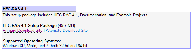
Select
the Primary Download Site and use Run as the option on the resulting
download package. You’ll see the Install
Wizard appear:
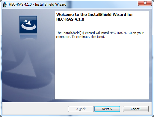
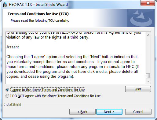
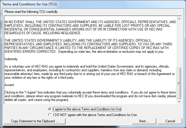
Hit
Next and you’ll get the Terms and
Conditions for Use and you have to scroll down to the bottom of the page of
these conditions before the “I agree to the above Terms and Conditions for Use”
button becomes selectable. Select this
button and hit Next.
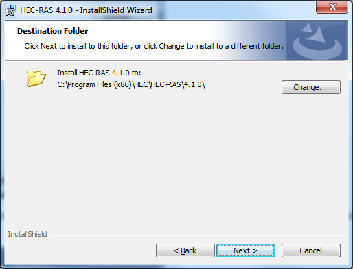
Select
a Destination Folder for the program files, or just let the program install it
in its default location (I normally just use the default location):
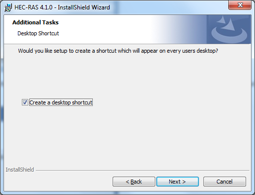
and
decide whether you want a Desktop Shortcut – this puts an icon on your Desktop
that allows you to directly open HEC-HMS without accessing your full programs
list. I usually select this option to
make the program easier to use.
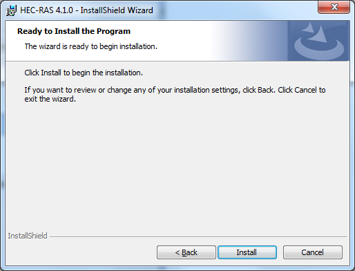
Then
Install the program, which takes a few minutes:
Once the program is installed, hit Finish to complete the Installation Wizard. Use the HEC-RAS icon to open the program:

If
you are the first user of this program, you’ll be prompted to agree to its
Terms and Conditions for use.
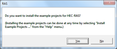
And
say “No” to installing the example projects for HEC-RAS.
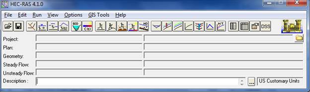
and
here is the opening screen of HEC-RAS.
2. Open existing
HEC-RAS Model
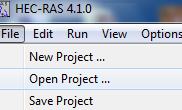
To
open an existing HEC-RAS model, click on RAS “File -> Open Project …” and
navigate to the UB100yr2.prj
file. This is a file for a HEC-RAS
model for the confluence of Brushy Creek and South Brushy Creek at Walsh Drive.
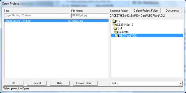
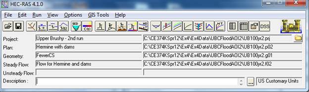
Hit OK to
load the project.
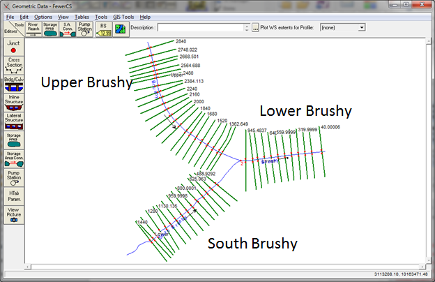
HEC-RAS
contains a series of Elements, and
in this project, lets start with the Geometric
Data. From “Edit” menu, select
“Geometric Data …”.
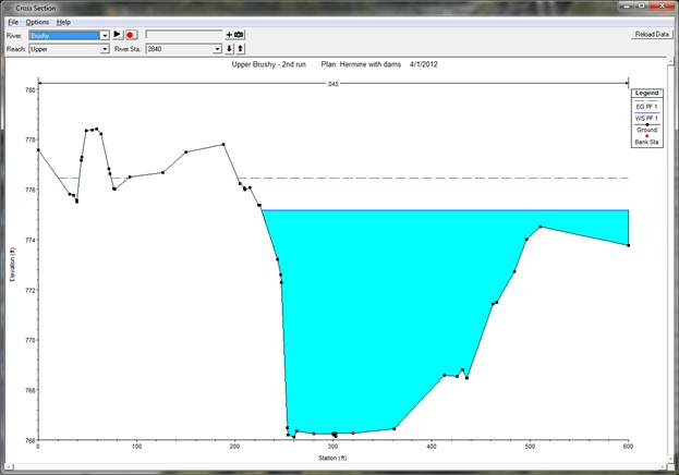
Open
the Cross-Section Editor ![]()
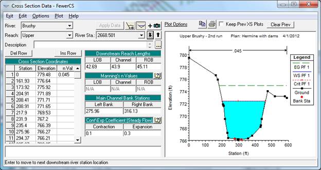
By
using the Up and Down arrows you can navigate along the
river cross-sections. By changing the Reach you can switch from Upper to
Lower Brushy Creek. By changing the River you can switch from Brushy Creek
to South Brushy Creek. Examine the
cross-sections in the model.
The
River Station gives the distance in
feet from the most downstream end of the River.
In this case 2668.501 feet is the distance from this cross-section on
Brushy Creek to the most downstream point on this creek shown in this model.
To be turned in: Determine the distance in feet from the
upper most to the lower most cross-section on Brushy Creek. How many cross-sections are there in this
distance? What is the average distance
between the cross-sections? Repeat this
calculation for South Brushy Creek.
Describe in words the cross-section at Station 2668.501 on Brushy
Creek. What value of Manning’s n is
used? What is the distance to the next
downstream cross-section (ft) for the Left Overbank, Channel and Right Overbank
flows? What is the lowest elevation of
the stream bed (ft above datum)? What is
the highest elevation of a point in the cross-section? What is the horizontal length of the
cross-section (ft)?
Close
the Geometric Data window.
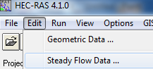
Now,
let’s review the steady flow data. From
“Edit” menu, select “Steady Flow Data …”.
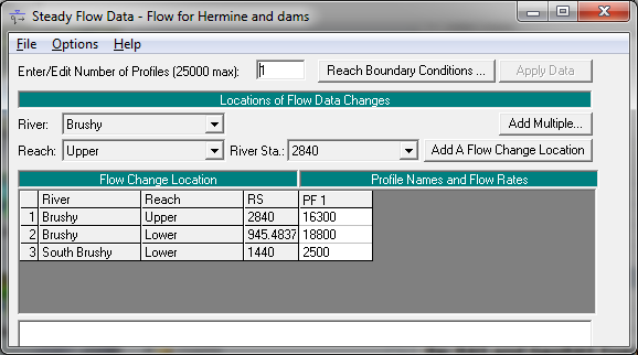
These
flows are approximated values taken from the HEC-HMS model for the flows during
Tropical Storm Hermine on Upper Brushy Creek.
The Lower Reach has the total flow of 18,800 cfs, which is divided into
16,300 cfs for the Upper Reach of Brushy Creek and 2500 cfs for the South Brushy
Creek (the flow that comes from Dam 7).
If you click on the box that says “Reach Boundary Conditions” you’ll see
a display like that shown below. What
this means is that at the downstream end of the lower reach, the Boundary
Condition is set at the Normal Depth for a bed slope of 0.008. The other two reaches have their downstream
boundary condition for depth equal to the upstream depth of the Lower Reach of
the main Brushy River.

Close
the Steady Flow Data window.
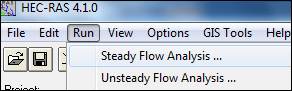
Frim
HEC=RAS “Run” menu select “ Steady Flow
Analysis …
The
Steady Flow Analysis form shows.
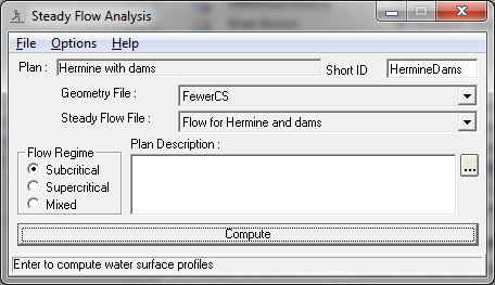
Click
on Compute. The model will run.
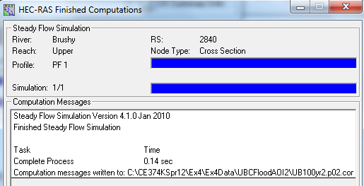
Close
the run and Steady Flow Analysis forms.
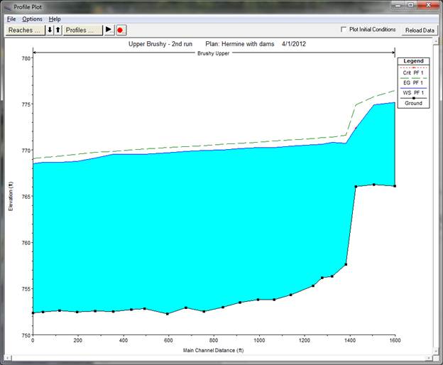
Click
on View profiles button (![]() ) on HEC-RAS interface. Review lingitudinal profiles fo rthe three
stream sections.
) on HEC-RAS interface. Review lingitudinal profiles fo rthe three
stream sections.
Click
on View cross sections button (![]() ) on HEC-RAS interface. Review cross-sections and water surface
elevations at cross-sections.
) on HEC-RAS interface. Review cross-sections and water surface
elevations at cross-sections.
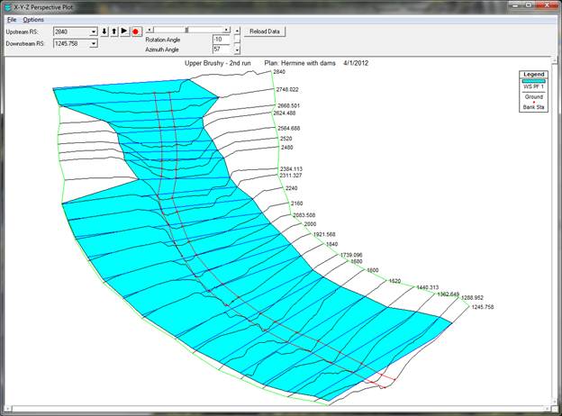
Click
on View 3D multiple cross section plot
button (![]() ) on HEC-RAS interface. Review cross-sections and water surface
elevations at cross-sections.
) on HEC-RAS interface. Review cross-sections and water surface
elevations at cross-sections.
Click
on View summary output tables by profile
button (![]() ) on HEC-RAS interface. Review results.
) on HEC-RAS interface. Review results.
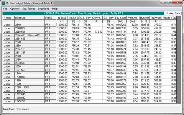
Change
the Profile Plot and then open the Summary Output Table for the new profile to
get the three tables describing the water surface profile in the three reaches.
To be Turned in: Calculate the average velocity over all
cross-sections in each of the three reaches (ft/sec). Using these data and the plots of the water
surface profiles, describe what is controlling the water surface elevation in
South Brushy Creek for the reach we have analyzed.
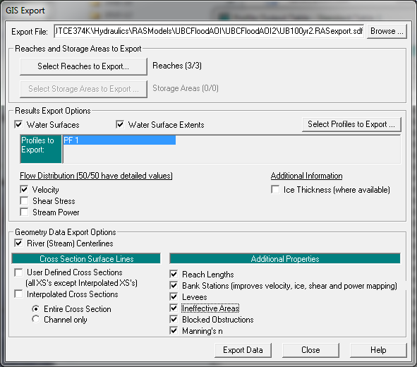
4. Export results to GIS format
From HEC-RAS “File” menu select “Export GIS Data …”.
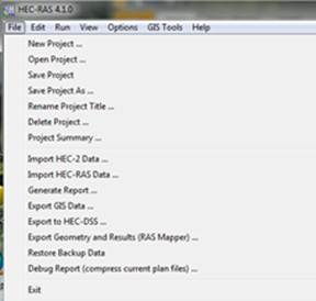
Populate the form and export the data.
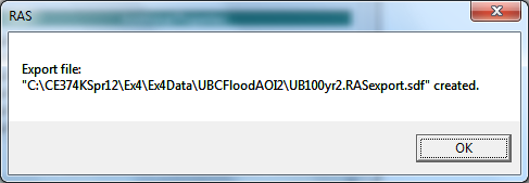
And you’ll see that this file has been created:
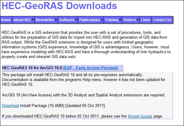
Now we need to get the HEC-GeoRAS extension for ArcGIS. If you’ve not already done this, go to http://www.hec.usace.army.mil/software/hec-ras/hec-georas.html and use Download to get the HEC-GeoRAS download for ArcGIS 10.0. There is also a Users Manual to HEC-GeoRAS at http://www.hec.usace.army.mil/software/hec-ras/documents/HEC-GeoRAS_43_Users_Manual.pdf
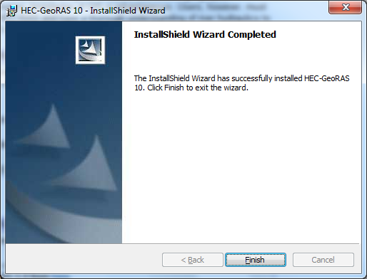
Go through the installation steps the same as for HEC-RAS.
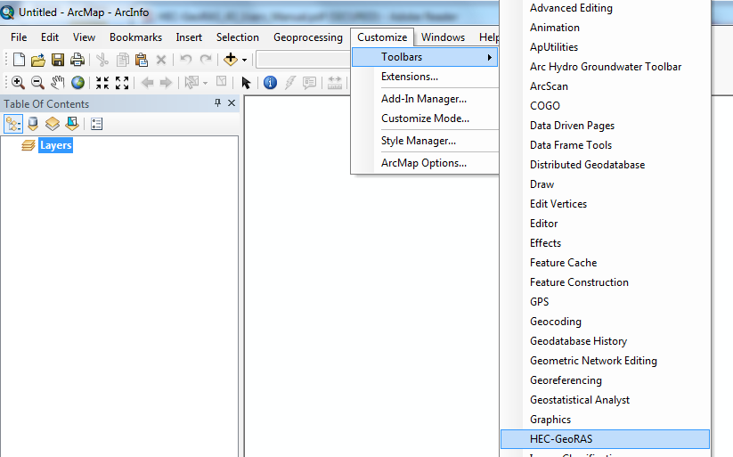
Open ArcGIS and in Customize Toolbars, select the HEC-GeoRAS option.
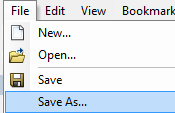
Save the ArcMap document as BrushyCreek.mxd
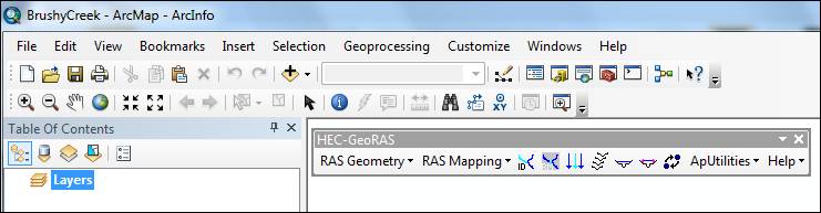
Here is what the ArcGIS display looks like with the HEC-GeoRAS extension loaded:
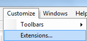
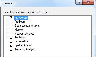
You need to have the Spatial Analyst and 3D Analyst extensions of ArcGIS to run this tool. You can check whether you have these extensions by using Customize/Extensions
Open an existing ArcMap GeoRAS project. Make sure GeoRAS toolbar is active. Save the project.
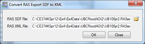
Click on “Import RAS SDF File” button (![]() )
from GeoRAS toolbar (this step converts the sdf file into an XML formatted file – it does not actually
import the data).
)
from GeoRAS toolbar (this step converts the sdf file into an XML formatted file – it does not actually
import the data).
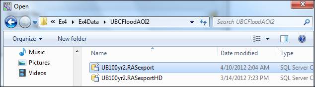
Select the sdf file created in previous step (this is of “RASExport” type). Note the name of the output file (same as the input file but with xml extension). Click on OK to perform the format conversion.
Don’t worry about an error message saying that this XML file already exists.
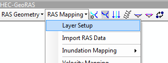
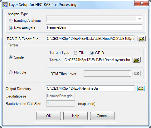
Define the new import project by running Layer Setup (from “RAS Mapping” menu on the GeoRAS toolbar).
Define:
i. Name of the new analysis (HermineDam)
ii. Name of the RAS GIS export file (UB100yr2.RASexport.XML)
iii. Which terrain dataset to use (ubcaoi).
iv. Output directory
v. Rasterization cell (accept default)
vi. The completed form should look like the following figure.
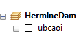
Click on OK. A new data frame will be created with the name matching the name of the analysis, with the specified terrain dataset loaded in it. The actual import of the data has not been performed yet. (The terrain is turned off by default, so the new data frame will appear empty).
Save the project.
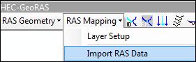
Import GIS data (“RAS Mapping -> Import RAS Data”). The process might take few minutes depending on the complexity of the results. During the process, several informative messages will be displayed in the form.
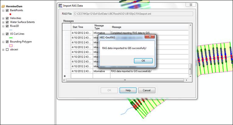
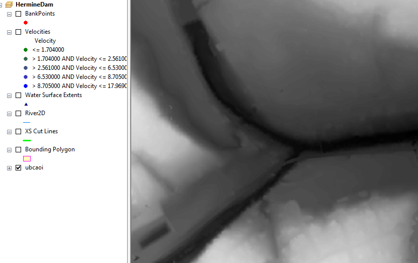
GIS representation of the BankPoints, Velocities, Water Surface Extent, River2D centerline, XS Cut Lines (these are the lines that were cut on the Digital Elevation Model to get the original cross-sections, the Bounding Polygon around the dataset. Explore the created dataset.

If you turn on only the DEM, ubcaoi, here is what you will see. UBCAOI stands for Upper Brushy Channel Area of Inundation.
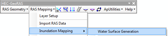
Create water surface TIN (water surface bound only by the extent of the bounding polygon) by running Water Surface Generation function (from “RAS Mapping -> Inundation Mapping” menu). TIN stands for Triangulated Irregular Network, which is another way that GIS uses to form surfaces by connecting points and lines into triangles.
a. Select the profile for which to create the water surface TIN. In our case there will be just one profile (PF1).
b. Check “Draw Output Layers” if you want to display the TIN (you might not want to do that if you select many profiles to generate at one time).
c. Select other options for smoothing and merging floodplain polygons (normally, keep these options unchecked).
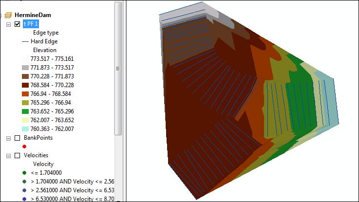
Here is the resulting TIN.
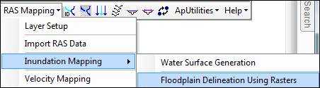
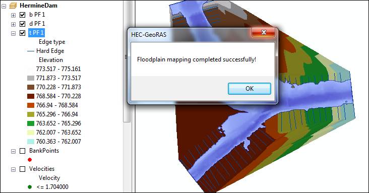
Generate floodplain and water depth (by running “RAS Mapping -> Inundation Mapping -> Floodplain Delineation Using Rasters” function).
a. Select one or several profiles for which to create the floodplain extent (depth grid will be created automatically). Only those profiles processed in step one will be available for processing.
b. Check “Draw Output Layers” if you want to display the output layers.
c. Check “Smooth Floodplain Delineation” if you want to smooth the output floodplain polygon (but you should not do that in the initially).
d. For each selected profile, a depth grid and a floodplain polygon feature class will be created.
And the following result appears!! What is happening here is that the TIN of the water surface is converted to a grid, and then the grid of the land surface elevation is subtracted from it to form the grid of the water depths shown below.
Review the results. Relate the floodplain shape and behavior to the assumptions of 1-D flow in RAS. Pay special attention to the following:
a. Where floodplain polygon extends all the way to the bounding polygon. This might indicate locations where cross-sections were not defined wide enough.
b. Where there is a break in floodplain polygon. This might indicate that cross-sections were not placed close enough.
c. Where there are isolated flooded areas (either on the cross-section or not). This might indicate isolated areas that should not be included as the flow contributing areas.
d. Where there are “flares” in the floodplain.
e. Where flow path lines (used to determine distances between cross-sections) are not within the floodplain.
f. If water surface extent points are not on the floodplain boundary.
g. Other unusual floodplain features.
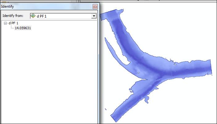
If you use the Identify tool ![]() on the layer d PF 1, you can check values of
the grid of the water depth.
on the layer d PF 1, you can check values of
the grid of the water depth.
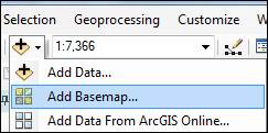
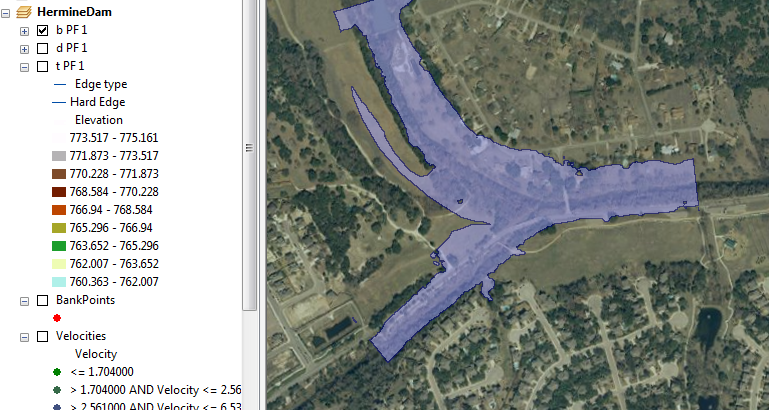
To provide some perspective of the background to this analysis, lets add a Basemap:
Choose the option for Imagery
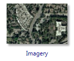
And you’ll get a rather nice display of the floodplain drawn over a map of Brushy Creek near Walsh Dr.
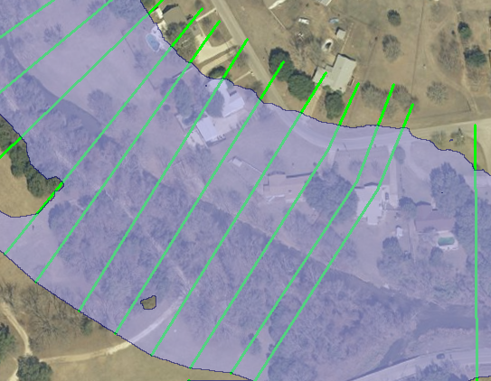
If you turn on the XS Cut Lines and zoom in you can see a rather nice map of the floodplain and the cross-sections used to create it in the neighbourhood of the homes we visited when we were on our field trip earlier this semester. Pretty cool!
To be turned in: A map showing the floodplain of Brushy Creek
in the area of Walsh Dr.
Summary of items to be turned in:
1. Determine
the distance in feet from the upper most to the lower most cross-section on
Brushy Creek. How many cross-sections
are there in this distance? What is the
average distance between the cross-sections?
Repeat this calculation for South Brushy Creek. Describe in words the cross-section at
Station 2668.501 on Brushy Creek. What
value of Manning’s n is used? What is
the distance to the next downstream cross-section (ft) for the Left Overbank,
Channel and Right Overbank flows? What
is the lowest elevation of the stream bed (ft above datum)? What is the highest elevation of a point in
the cross-section? What is the
horizontal length of the cross-section (ft)?
2.
Calculate the average velocity over all cross-sections in each of the
three reaches (ft/sec). Using these
data and the plots of the water surface profiles, describe what is controlling
the water surface elevation in South Brushy Creek for the reach we have
analyzed.
3.
A map showing the floodplain of Brushy Creek in the area of Walsh
Dr.
Ok, you’re done!