Exercise
2. Energy Balance of the
CE
394K.2
Spring 2007
Revised Version: 13 February 2007
Prepared by David R. Maidment, Jon Goodall
and Cédric H. David
Table of Contents
Computer and data requirements
Procedure
1. Making the link to NARR data in IDV
4. Map display of the San Marcos basin
5. netCDF files in ArcGIS 9.2, energy balance in the San Marcos BasinData
Goals of the Exercise
The goals of this exercise are for you to become familiar with the Integrated Data Viewer as a way of viewing and querying atmospheric science datasets for the energy balance of the earth, and to construct an energy balance for a typical day in July 2003 for North America, and for a location 30.02ºN and 98.2ºW in the San Marcos basin, using ArcGIS 9.2 capabilities.
Computer and Data Requirements
Integrated Data Viewer
The
Integrated Data Viewer (IDV) is developed by Unidata (http://www.unidata.ucar.edu/) a program
of the Universities Corporation for Atmospheric Research located in
For this exercise, we are going to use historical weather model data from the North American Regional Reanalysis (NARR), http://wwwt.emc.ncep.noaa.gov/mmb/rreanl/index.html which is an archive for 1979 to present developed by running the Eta numerical weather prediction model of the National Centers for Environmental Prediction on an historical database of weather observations.
To be turned in: Make a brief summary of the North American
Regional Reanalysis – how was it produced, what data summaries does it contain,
what is its spatial extent and coverage in time?
1. Making the link to NARR data in IDV
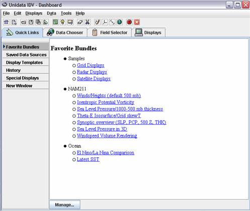
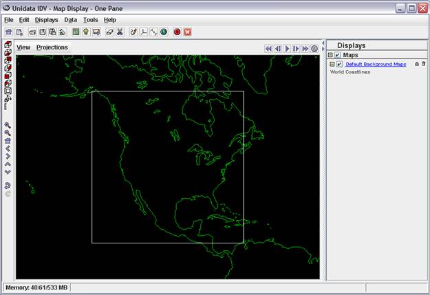
Open IDV by using the same link that was used to install it (http://www.unidata.ucar.edu/software/idv/webstart/IDV/idv.jnlp). Two Java windows will open: the Dashboard and the Map Display.
In
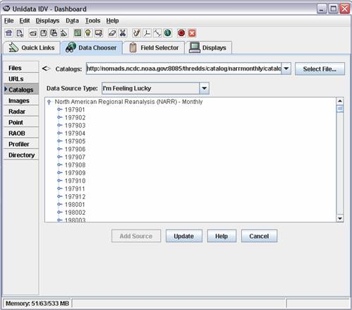
the Dashboard, select Data Chooser / Catalogs and paste the following link: http://nomads.ncdc.noaa.gov:8085/thredds/catalog/narrmonthly/catalog.xml.
Make sure that you have Catalogs highlighted in the left pane
of the screen below before you do the paste of the catalog.xml location. 
Then
hit Update on the button at the
bottom of the screen so that you connect to the data source. You are viewing files resident at the
Scroll down to July 2003 and expand, you should see the following:
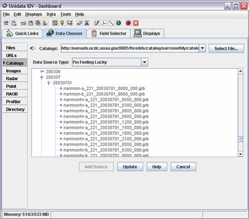
You are viewing files from the NARR monthly dataset for the month of July 2003.
Note: by using the higher hierarchy catalog: http://nomads.ncdc.noaa.gov:8085/thredds/catalog.xml, you will have access to multiple datasets served by NCDC.
NARR-B Monthly has energy data, let's give a
look at narrmonhr-b_221_20030701_1200_000.grb, this file has 3-hour averaged data
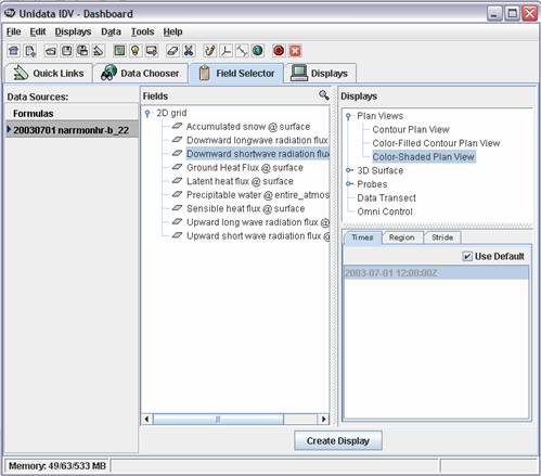
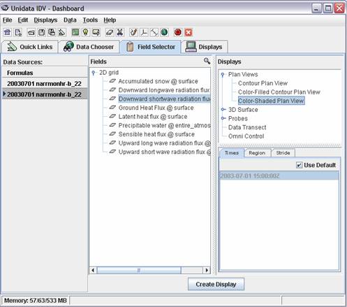
(from 1200 hours to 1500 hours for every day of July 2003). Double click on at narrmonhr-b_221_20030701_1200_000.grb, the Dashboard will
automatically transfer to its Field
Selector tab.
Expand 2D
grid, select Downward shortwave wave
radiation flux, and Color-Shaded
Plan View. Then click on Create Display
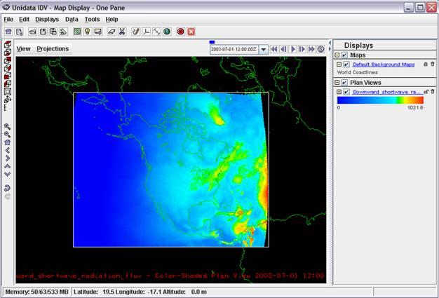
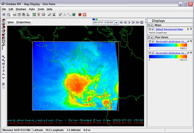
The following Map Display will appear
(totally cool!!)
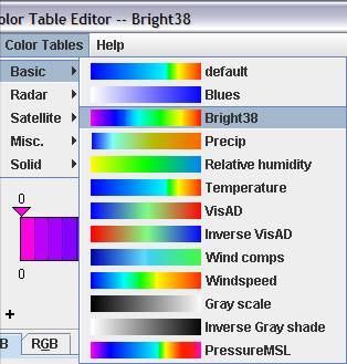
In order to be able to compare multiple
files, we need to make the color tables similar. Click on the color table, the Color Table Editor window will open:

Select Color Tables / Basic / Bright38 as the color table, then set
the range to 0 – 1200. Hit Apply at the bottom of the Color Table Editor. The
units of downward shortwave variation flux are W / m2.
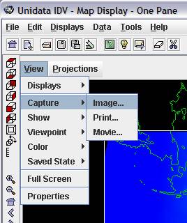
You can capture your display using View, Capture, Image and save
as a jpg file.
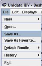
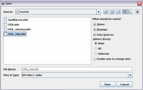
It's good at this point to save the display
you’ve created. To do this, use File/Save As from the main IDV Window and
save the file as USA_July.xidv. The
extension .xidv is a signal that this is an IDV map file.
By repeating the same display process with
the other 3-hour intervals of July 2003, you will be able to see the estimated
downward shortwave (solar) radiation for a given hour averaged across all the
days of July 2003. In the Dashboard, select the Data Chooser tab. Double click on another 3-hour interval, narrmonhr-b_221_20030701_1500_000.grb
for example.
You should see the following display:
Make all July displays for downward shortwave
radiation flux and color them similarly.
You can get rid of the unwanted displays with the little garbage can on
the right hand side of the legend display.
![]()
To
be turned in: Make a display of the
downward solar radiation for each of the 3 hr intervals for July 2003 and make
a similar series of 8 maps for January 2003.
At what Z time does the maximum solar radiation occur? Where is the maximum solar radiation located
for January? Where is the maximum solar
radiation for July? The data you are viewing
are solar radiation at ground level, not at the top of the atmosphere. Why is there more solar radiation in the
western US during July than in the eastern US?
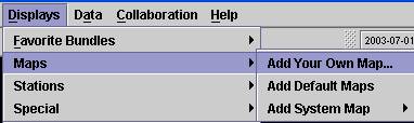
4. Map Display of the
Now let's focus in on the
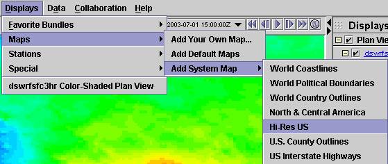
and you’ll get a display with the Hi-Res US
like below.
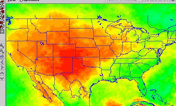
You can use the zoom and arrow tools on the
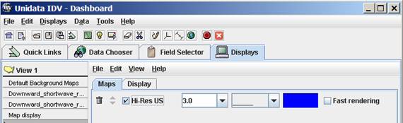
left side of the display to zoom in and center your picture. If the color of an added map is not what you
want, click on Map Display ![]() to bring up an editor that lets you change the
map colors. If you don’t see the display
at all, click on Map display and make sure that the Hi-Res US is clicked on
to bring up an editor that lets you change the
map colors. If you don’t see the display
at all, click on Map display and make sure that the Hi-Res US is clicked on ![]() (the default is that it is clicked off) and
then you’ll see the Hi-Res map display.
(the default is that it is clicked off) and
then you’ll see the Hi-Res map display.
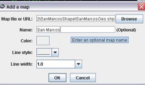
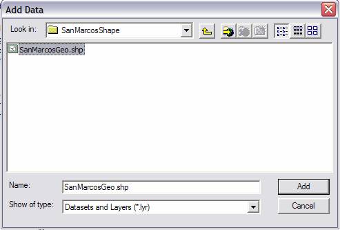
To add a map of the
You’ll get a display that says “Add a Map”,
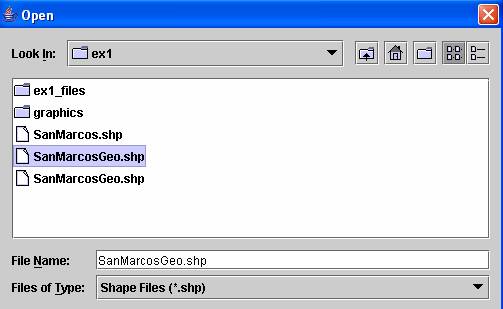
hit the Browse button
and you’ll get a new window that says Open, Select Files of Type Shape Files (*.shp) at the bottom of the page
and you can select individual shape files.
You can then rename the map to
Note that maps must be in geographic coordinates to display correctly in the
IDV. You can zoom in on a view of the
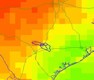
It’s a good idea to use File/Save As to resave your IDV map images now.
To
be turned in: A map display showing the
5. netCDF files in ArcGIS 9.2,
energy balance in the
ArcGIS 9.2
The latest version of ArcGIS has the capability of reading netCDF files. NetCDF are very common in atmospheric sciences.
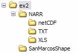
Data Files
The data files for this exercise are available at ex2.zip. They consist of:
·
NARR data in netCDF, text and Excel format, for
the
·
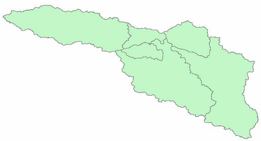
A Shapefile of the
This portion of the exercise assumes that you
know how to use ArcMap. If you don’t,
please refer to Exercise 1 of my GIS in Water Resources class for an
introductory tutorial on using ArcMap: http://www.ce.utexas.edu/prof/maidment/giswr2006/Ex1/Ex12006.doc
Until now, all the files we have viewed
remained on the server at NCDC and were not downloaded to your local
machine. In order to be able to use the
ArcGIS 9.2 environment, netCDF files need to be downloaded on your
computer. This task has already been
accomplished for you (for July 2003); the files are available in ex2 / NARR / netCDF. If interested in downloading the files
yourself, please refer to the tutorial http://www.ce.utexas.edu/prof/maidment/GradHydro2007/docs/NetCDF_Unidata.pdf
Let's now open netCDF files in ArcGIS 9.2! Very cool new stuff!
Open ArcMap,
add the SanMarcosGeo shapefile.
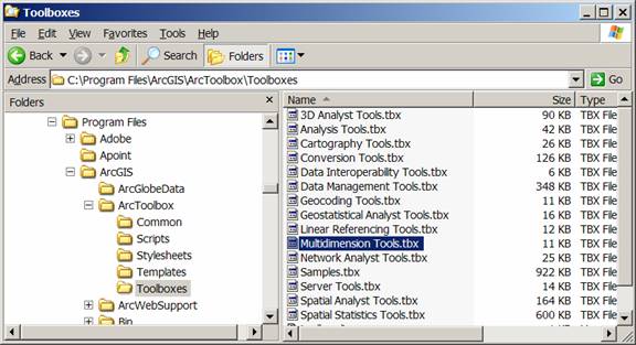
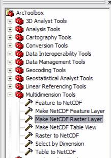
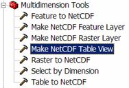
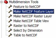
Open Arc Toolbox by hitting the ![]() button in the ArcMap toolbar. You need the Multidimension Tools.
button in the ArcMap toolbar. You need the Multidimension Tools. ![]() If you
don’t see this option in your ArcToolbox display you can add it (provided you
are using ArcGIS 9.2) by right clicking in the white space in the Arc Toolbox
area and navigating to the toolbox folder in the ArcGIS program files. I found
it at the following location:
If you
don’t see this option in your ArcToolbox display you can add it (provided you
are using ArcGIS 9.2) by right clicking in the white space in the Arc Toolbox
area and navigating to the toolbox folder in the ArcGIS program files. I found
it at the following location:
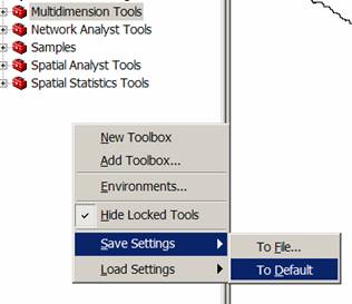
To ensure that you will have the
Multidimension Toolbox displayed the next time you open ArcGIS, Right click on
the white space below the tools in Arc Toolbox and select Save Settings… To Default, as shown below:
Use the Multidimension
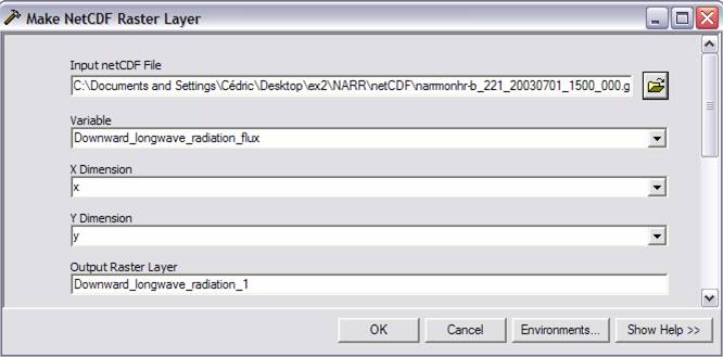
tools / Make netCDF raster layer:
Browse to your netCDF file, here narrmonhr-b_221_20030701_1500_000.grb.nc is
given as an example. Select the variable
desired, and keep all the other parameters as default.
Click OK, you should see the following
screen:
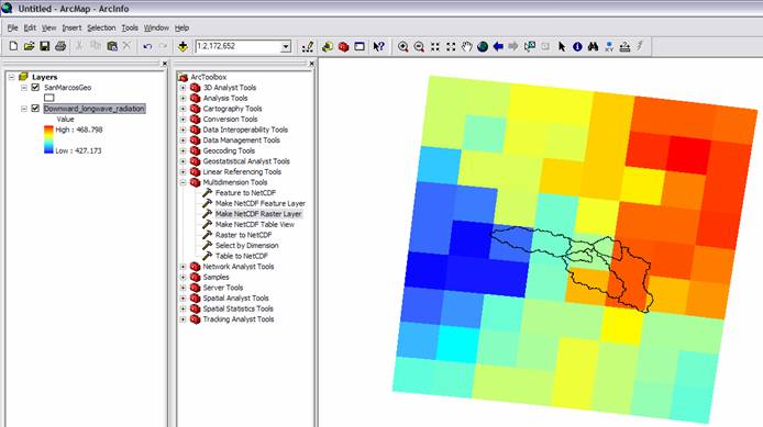
You just created a raster display of a netCDf
file in ArcGIS 9.2! There are a total of
72 cells shown in this display, 9 upwards and 8 across, and by viewing the Layers
in a Projected Coordinate system, you can find out that the size of the cells
is approximately 30.5 km x 30.5 km, or 92 km2.
We are now going to perform an energy balance
for one point in the

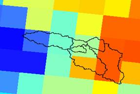
The center of the grid shown above
corresponds to 30.0°N and 98.2°W, also symbolized with a circle in the picture
below. Add to your display Downward and
Upward Shortwave radiation flux, Downward and Upward Longwave radiation flux,
and Sensible, Latent and Ground Heat flux, a total of seven flux components,
order them as shown in the map display below, and use the Identify tool in
ArcGIS to query <All Layers> in the map display. You’ll get a sequence of values in the query
tool for the 7 components of the energy balance, as shown.
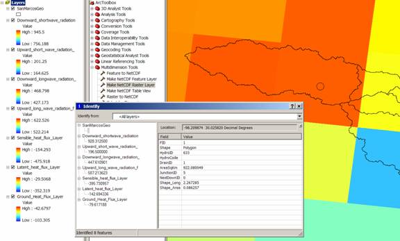
If you
transpose these values to Excel, you can make a table and a graph of the energy
balance at this time interval (1500Z).
Now to translate that into local time, we subtract 5 hours because July
is when we are using Central Daylight Time (we would subtract 6 hours if this
were January because then we are using Central Standard Time), and we recognize
that these data represent an average over a three hour time interval, so what
you are looking at this an energy balance from 10AM to 1PM Central Daylight
Time in the San Marcos Basin (actually the Blanco watershed near Wimberley,
Texas).
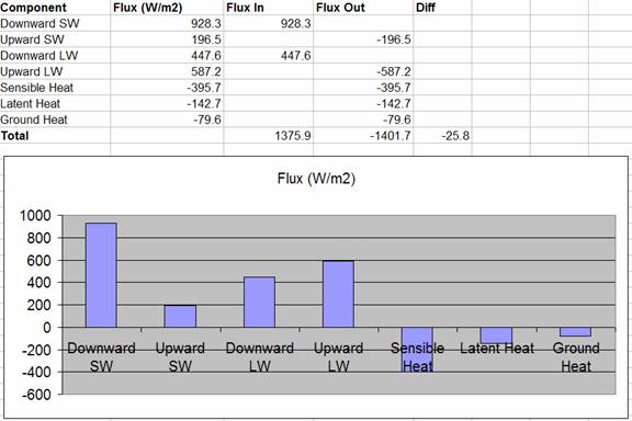
It requires some interpretation to figure out
what all the signs mean here. What we
are doing is working out the energy balance on a unit area of the land surface,
say 1 m2. The downward Short
Wave flux is that which comes from the sun, the upward Short Wave flux is that
reflected from the land surface, so in this instance, the surface albedo is
196.5/928.3 = 0.21. The Downward
Longwave is that which comes from reradiation from the clouds and atmosphere
and Upward Longwave is the reflected component plus the emission of longwave
radiation by the earth itself (which is why the Upward LW is larger than the
Downward Longwave). The Sensible Heat is
that which goes to heat the air, the Latent Heat is that which evaporates water
and the Ground Heat is that which is heating the soil. These last three quantities (Sensible,
Latent and Ground Heat) are considered negative when they take heat away from
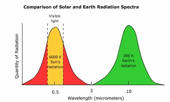
the land surface. Shortwave radiation is
that less than 3 mm in wavelength and
Longwave radiation is that greater than 3 mm
as indicated in the radiation diagram below.
You can make an energy balance by considering
all radiation quantities that bring energy flux
in to the land surface as positive and all those that have an energy flux out from the land surface as
negative, as indicated in the spreadsheet above. Now, in theory, all these quantities should
sum to 0 but you can see that there is a small discrepancy here of about 25 W/m2.
ArcGIS 9.2 allows you to create rasters,
features, and tables out of netCDF files.
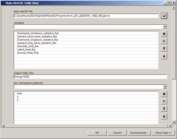
Lets make a table. Choose the Make NetCDF Table View and navigate to
the same file for 1500Z that you were using before: narrmonhr-b_221_20030701_1500_000.grb.nc
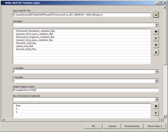
In the Variables
scroll box you’ll see all the radiation components. Select them one at a time and use the + button ![]() to add them to the Table View. Lets call the Output Table, Energy1500Z.
to add them to the Table View. Lets call the Output Table, Energy1500Z.
Add in the Scrolldown box at the bottom the
Row dimensions Time, X, Y. If you don’t
do this you will only get one record added to your table rather than all of
them.
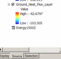
Now if we change the ArcMap Legend tab from Display to Source, the Energy1500Z table shows up.
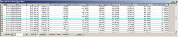
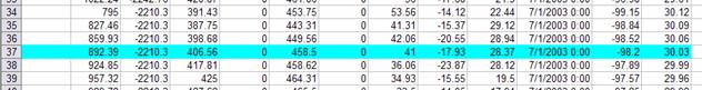
If you open the resulting table, you’ll see
72 rows of energy balance information, with the cell you examined in row 35:
Ok, this is starting to be a lot of
information. You can see how netCDF can
start to bring some considerable additional detail to our understanding of the
landscape. We can also view netCDF files
as features, using the Make NetCDF
Feature Layer. Proceed as before
with the selection of variables and rows.
And the result displays as:

Ok, this is a lot clearer. You can see a point at the center of each
cell and if you query the point at the center of the cell we’ve been working
on, you can see all the same flux components that we have already
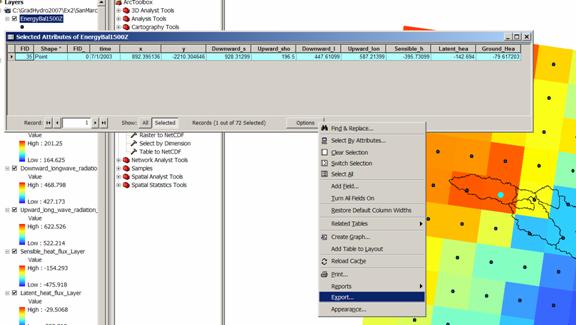
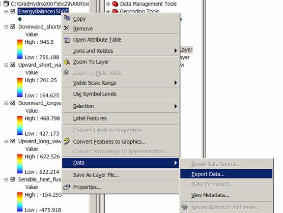
examined. To store these data
permanently, right click on the EnergyBalance1500Z layer and say it as a shape file. Then you can re-add it to the map, select the
point we are interested in, and export its data only to a .dbf file and thus
import it into Excel.
With a process similar to the previous,
tables can be created and exported as text files, and can be imported into
Excel. This process has aready been
accomplished for you and text and Excel files corresponding to the netCDF files
in ex2 / NARR / netCDF can be
found in ex2 / NARR / TXT and ex2 / NARR / XLS.
The
data corresponding to this point has been highlighted in all the Excel files
given.
Here
is a plot of daily average values of the flux components for the month of July
2003: 
The upward longwave and shortwave components have been made negative in this plot to indicate that they are energy losses from the earth’s surface. Net radiation = DownSW + DownLW – UpLong – UpShort. This net radiation is consumed by ground heat flux (G), latent heat flux (L) and sensible heat flux (S). The balance is the sum of the net radiation and G + L + S. It should theoretically go to 0.
To
be turned in: Make a table showing the
Downward Short Wave Radiation values for 30.0°N and 98.2°W for each three hour
interval during the day in July. Make a
similar listing for the values of
1.
Downward Longwave Radiation Flux
2. Downward Shortwave Radiation Flux
3. Ground Heat Flux
4. Latent Heat Flux
5. Sensible Heat Flux
6. Upward Long Wave Radiation Flux
7. Upward Short Wave Radiation Flux
Calculate
the energy balance for 30.0°N and 98.2°W.
Make
graphs showing data series 1-7 as a function of time of the day.
What
is average July evaporation in mm/day at this location?
Choose
a different box of the 72 boxes located in the
Now, if you want to get your own data for
another part of the country, you can go to:
http://nomads.ncdc.noaa.gov:8085/thredds/catalog.html
in a web browser and find additional files.
Ok, you’re done!
Summary of items to be turned in
To be turned in: Make a brief summary of the North American
Regional Reanalysis – how was it produced, what data summaries does it contain,
what is its spatial extent and coverage in time?
To
be turned in: Make a display of the
downward solar radiation for each of the 3 hr intervals for July 2003 and make
a similar series of 8 maps for January 2003.
At what Z time does the maximum solar radiation occur? Where is the maximum solar radiation located
for January? Where is the maximum solar
radiation for July? The data you are
viewing are solar radiation at ground level, not at the top of the
atmosphere. Why is there more solar
radiation in the western US during July than in the eastern US?
To
be turned in: A map display showing the
To
be turned in: Make a table showing the
Downward Short Wave Radiation values for 30.0°N and 98.2°W for each three hour
interval during the day in July. Make a
similar listing for the values of
1.
Downward Longwave Radiation Flux
2. Downward Shortwave Radiation Flux
3. Ground Heat Flux
4. Latent Heat Flux
5. Sensible Heat Flux
6. Upward Long Wave Radiation Flux
7. Upward Short Wave Radiation Flux
Calculate
the energy balance for 30.02°N and 98.2°W.
Make
graphs showing data series 1-7 as a function of time of the day.
What
is average July evaporation in mm/day at this location?
Choose
a different box of the 72 boxes located in the