A 5 km precipitation grid, a 500 m digital elevation
model (DEM), gaged streamflow data, and other data sets were used
to generate spatially distributed maps of mean annual runoff and
evaporation for the state of Texas. In the process of creating
these maps, 166 gaged watersheds were delineated and a set of
hydrologic attributes was compiled for each watershed including
net measured inflow, precipitation, reservoir evaporation, recharge,
urban landuse fraction, and springflow. To estimate the runoff
in ungaged locations, a curve of "expected" annual runoff
as a function of rainfall was developed. The term "expected"
refers to runoff that occurs under normal or natural conditions.
In other words, watersheds with unique hydrogeology that exhibit
unusually large recharge or springflows were removed from consideration,
as well as watersheds with a large amount of urban development,
and watersheds with significant reservoir evaporation.
The terms large and significant are described by
a set of criteria developed using GIS data layers.
An equation fitted to the expected rainfall-runoff
curve was applied to each cell in the precipitation grid to generate
an expected runoff grid. For gaged watersheds, the difference
between the actual runoff per unit area and the expected runoff
per unit area was computed, and these values (one per watershed)
were used to create an adjustment grid. The adjustment grid has
a 500 m cell resolution so that watersheds delineated at this
threshold and 5 km cell information could be combined. Adding
the adjustment grid to the expected runoff grid results in a grid
of actual runoff. This method forces the sum of cells in the
actual runoff grid within each watershed to equal the net measured
inflow for that watershed. In ungaged areas, the actual runoff
was assumed to be equal to the expected runoff. By applying a
flow accumulation function to the runoff maps, the expected and
actual flows were calculated at each 500 m DEM cell in Texas and
flow maps were created.
Using the assumption that the change in annual watershed
storage is zero, a grid of losses was created by subtracting the
runoff grid from the precipitation grid. This grid can be interpreted
as a grid of evaporation except in locations where there is significant
inter-watershed transfer (Edward's Aquifer flowing to Comal Springs
for example). Inter-watershed transfer, of course, depends on
which watersheds are delineated.
In this study, rainfall and streamflow data were
averaged over the time period 1961-1990. The reason for choosing
this time period was that 2.5 minute grids of mean annual and
mean monthly rainfall representative of the 1961-1990 period are
available for the entire United States. These grids were created
at Oregon State University using the PRISM model for interpolation
(Daly et al., 1994).
Accomplishing the tasks described above involved
a large amount of data processing using ArcView GIS with Avenue,
Arc/Info GIS, and FORTRAN. Major steps in the analysis included
(1) DEM processing, (2) selecting a set of flow gages spanning
the appropriate period of record, (3) delineating watersheds from
selected gages, (4) determining the average annual precipitation
in each watershed, (5) determining the net measured inflow to
each watershed, (6) compiling a set of watershed attributes including
percent urbanization, reservoir evaporation, recharge, and springflow,
(7) plotting runoff per unit area versus rainfall per unit area
and deriving an "expected" runoff function, and (8)
creating grids of expected runoff, actual runoff, and evaporation.
5.2.1 Digital Elevation
Model Processing
Two digital elevation models (DEMs) were used for
defining watersheds in this study. The portion of the 15"
USGS DEM covering the conterminous United States that either falls
within or drains to Texas was clipped for use in this study.
To approximate the Rio Grande drainage contribution from Mexico,
a piece of the 30" USGS DEM of North America was merged with
the 15" DEM. A 15" DEM corresponds to approximately
500 m on the earth's surface and a 30" DEM corresponds to
approximately 1 km. To cover all areas draining to Texas a grid
of approximately 10 million cells was processed, although only
about 2.7 million of these cells actually fall within Texas.
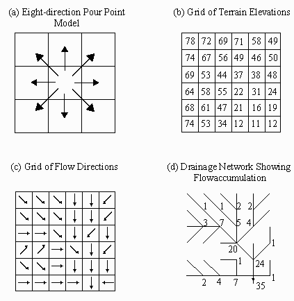
The eight direction pour point model is the basic
model that underlies watershed and drainage network delineation
with grid processing. As illustrated in Figure 5.1, the assumption
is that water in a given cell will flow towards only one of its
neighboring cells, whichever cell lies in the direction of steepest
descent. A Flowdirection function applied to an elevation grid
(Figure 5.1b) yields a grid of flow directions (Figure 5.1c).
From this grid of flow directions, a drainage network is derived
(Figure 5.1d). The flow accumulation is the number of cells upstream
of any given cell in the drainage network.

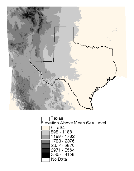
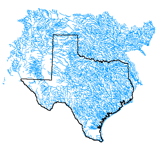
Before defining the drainage network using the eight direction pour point model, several processing steps were taken in order to create a "hydrologic" DEM from the raw DEM. First, the data from the two DEMs (Texas and Mexico) were merged into one grid. Next, the combined DEM was filled to remove pits. A pit is a cell or group of cells that is lower that all of its neighboring cells. Pits are removed so that there will be no discontinuities in the drainage network derived from the DEM; no internal drainage is allowed by this model. The DEM was also modified so that streams delineated from the DEM are consistent with digitized streams in EPA's River Reach File 1 (RF1). This process of DEM modification is referred to as "burning in the streams." The simplest stream burn-in procedure involves (1) creating a gridded representation of the digitized stream network (RF1) and identifying cells as being either stream cells or land surface cells, (2) raising the elevation of land surface cells relative to stream cells, and (3) deriving the drainage network based upon flow direction values defined by the burned DEM. Because many arcs in RF1 are not connected to the major river systems, burning in these arcs creates inland drainage basins or pits. Some of these disconnected arcs may represent real inland drainage basins or playas; however, information as to where inland drainage occurs was not readily available, so the DEM was filled a second time to eliminate pits created by the burning procedure. One drawback of the DEM analysis used here is that non-contributing drainage areas are considered as contributing to downstream runoff. This may cause the runoff per unit area estimates in some watersheds to be too low; however, the runoff total at watershed outlets is still consistent with measured flows. Figure 5.2 is a map showing the processed DEM and Figure 5.3 is a map showing RF1 streams.
The flow direction and flow accumulation grids derived
from the burned DEM were used to delineate watersheds and streams.
A grid of stream cells contains those cells with a flow accumulation
greater than 1000 cells or 250 km2. Cells on this
stream network are candidates for selection as watershed outlet
cells. A 1000 cell threshold was chosen because watersheds delineated
with fewer than 1000 cells tend to be poorly defined. A grid
of stream links was also created using the stream network and
flow direction grids. In the stream link grid, each stream reach
is assigned a unique value. This is useful because each outlet
cell used to delineate watersheds needs to have a unique value
and outlet cells selected directly from the stream link grid satisfy
the criterion as long as there are not two gages along the same
reach. In this study, outlet cells were selected based upon the
location of USGS gaging stations. The manner in which stations
were selected for analysis is described in the next section.
5.2.2 Selecting Gaging
Stations for Analysis
All monthly and daily flow records for the water
years 1961 - 1990 and for all USGS gaging stations in Texas were
extracted from the Hydrosphere CD-ROM "USGS Daily Values
: West 2." The Hydrosphere software was used to write the
flow records for all Texas stations to a dBase file. This dBase
file also includes latitude, longitude, and other station information.
Because this dBase file is very large, with up to 360 records
for each of 693 stations, an Avenue script was used to extract
summary information for each station. The result is a dBase file
that contains only one record for each station. Key attributes
available for each station record are latitude, longitude, starting
year, ending year, 30-year mean monthly flows, and 30-year mean
annual flows.
From the list of 693 stations, stations operating
during the entire 1961-1990 period were selected, yielding a set
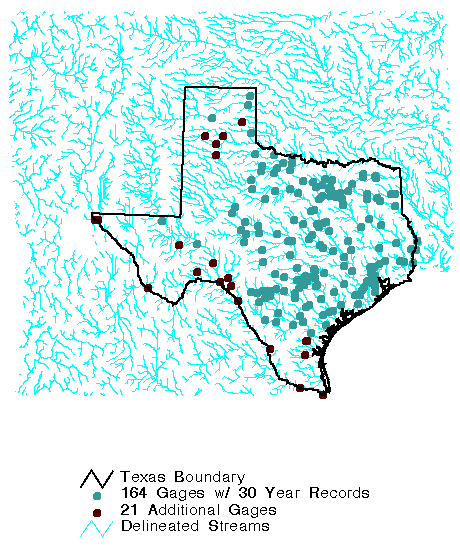
of 164 stations. Even with all 164 stations, there is almost
no coverage of the Rio Grande basin and sparse coverage of the
western part of the Red River basin; therefore, an additional
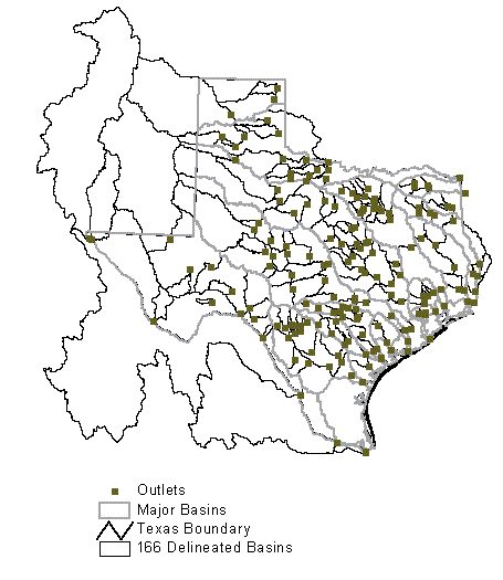
21 gages were selected to cover these areas. Figure 5.4 is a
map of station locations. Although these gages have incomplete
records for the 1961-1990 averaging period, the 30-year mean flows
were approximated by using an adjustment based on a nearby gage
with a complete record for this period. The following equation
was used for making flow adjustments:

In Equation 5.1, station b is a station with incomplete
records covering x years (x < 30) of the period from 1961 -
1990 and station a is a nearby station with complete records for
this period.
5.2.3 Watershed Delineation
Watershed delineation requires a grid of flow directions
and a grid of outlet cells. Deriving a grid of flow directions
was described in the above section on "DEM Processing."
Because the latitude and longitude coordinates of the USGS gaging
stations do not fall precisely on the gridded stream network,
some mechanism for choosing outlet cells is required. An AML
script that runs in Arc/Info Grid was used to select outlet cells.
This script takes a point coverage of gaging stations and a grid
of stream links as input. The script is interactive and works
in the following way: The program loops through the point coverage
and the vicinity of the current point (approximately ten cells
in each direction) is displayed. The user is then prompted to
select an outlet cell and after selection, the coordinates of
the selected cell are written to a text file. Using the output
text file, a point coverage of outlets can be created and this
point coverage converted to a grid of outlets. With this grid
of outlets and the flow direction grid, watersheds are delineated.
The reason for interactive selection of outlets is that some
user discretion may be required. In this study, watersheds with
a drainage area less than 250 km2 were not delineated,
resulting in the delineation of 166 watersheds.
After studying the watershed delineation, two correctable
errors in the delineation were found. The first error was that
part of the Red River Basin drained southward into the Rio Grande
Basin. This error was caused by the burn-in procedure the proximity
of two tributaries in RF1 that drain towards different basins
resulted in the creation of a ditch that crossed a ridge line.
This error was corrected by manually editing two cell values
in the burned DEM. The second error involves the delineation
of the Mexico portion of the Rio Grande. Although no counterpart
to the RF1 line work was available for Mexico, a comparison of
the delineated Rio Grande basin with a published map revealed
an extraneous area in Mexico (southwest of El Paso) draining towards
the Rio Grande. This problem appears to be caused because the
fill procedure filled an area that may actually be an inland drainage
basin or basins. The problem was corrected by editing a string
of cells in the burned DEM; however, this correction is only an
approximate visual correction and the accuracy of the resulting
delineation in defining the drainage area of the Rio Conchos tributary
of the Rio Grande is questionable. After these DEM edits were
made, the flow direction grid was re-calculated and the watershed
re-delineated. Figure 5.5 shows the delineated watersheds. For
reference, the fifteen major river basins in Texas were also delineated
using a similar procedure to that used for delineating all 166
watersheds.
A comparison was made between the drainage areas defined by the DEM and those reported by the USGS for each gage. Since the USGS reports total upstream drainage area, the USGS incremental drainage areas were computed for non-source watersheds. For all but 16 of the delineated watersheds, the DEM area is within 15% of the area reported by the USGS. This comparison is shown in Figure 5.6. The 16 watersheds with incorrect areas were not used in the analysis. The reasons for some of the worst discrepancies are obvious, and some of the discrepancies are clearly problems with using the DEM while others point to errors in the USGS values. For example, one station on the Sabine River has a USGS reported drainage area of about 19,000 km2 while an upstream station has a reported drainage area of 21,000 km2 which can't be true. In another situation, the USGS gage measures flow in a government ditch rather than a natural stream and DEM analysis cannot identify a government ditch. The drainage area of the Rio Grande from Mexico is suspect because of inaccuracies associated with using the 30" DEM. Despite these problems, the accuracy achieved using the 500 m DEM is satisfactory in most of the watersheds, especially since the total runoff predicted for each watershed (sum of the runoff in all cells) is forced to match that dictated by the gaging stations.
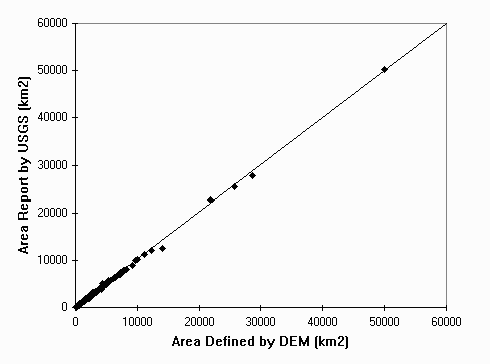
Figure 5-6: Watershed Areas Reported By USGS versus Areas Defined by DEM for All But 16 Watersheds
5.2.4 Compiling Watershed
Attributes
5.2.4.1 Determining Mean Precipitation and Net Inflow
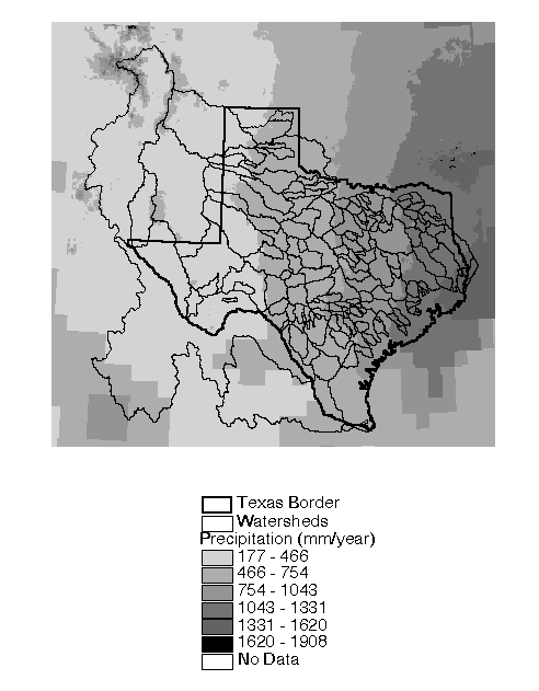
Given a grid of precipitation values and a grid of watersheds, a single Arc/Info Grid function (Zonalstats) creates a table of the mean precipitation in each watershed, provided the two grids are defined with the same cell size. Precipitation grids of the United States (2.5 arc-minutes) with mean monthly and mean annual values (approximately 5 km in projected space) were used in this study. The precipitation grids were resampled to a 500 m cell size to match the resolution of the watershed boundaries and enable the computation of watershed averages. Since the Mexico portion of the Rio Grande is not covered by these 2.5' grids, a global 0.5 data set obtained from Cort Willmott at the University of Delaware was used to fill in this space. The values in the Willmott grids were adjusted by a ratio to reflect the same climatic averaging period as that used to create the Oregon State grids. The combined grid of mean annual values is shown in Figure 5.7.
5.2.4.2 Reservoir Evaporation
Mean annual evaporation due to reservoirs in each of the 166 watersheds was estimated. The data used to make these estimates, reservoir evaporation data and a reservoir area, were provided by the Texas Water Development Board (TWDB). A text file containing monthly average gross reservoir evaporation estimates for 1 quadrangles in Texas was provided by Alfredo Rodriguez, TWDB, (personal communication, 1996). This text file contains monthly data for 1940 to 1990 in 75 quadrangles and monthly data for 1971-1990 in 28 quadrangles. The gross monthly evaporation data were written to an INFO file and the average potential reservoir evaporation for each year was computed, as well as the average reservoir evaporation for our 30 year study period 1961 - 1990 (or 1971 - 1990 for those quadrangles lacking records back to the 1960's). An Arc/Info coverage of the quadrangles was created and several attributes were joined to this coverage: TWDB identification number, starting and ending years for available data, mean reservoir evaporation from 1961-1990, and mean reservoir evaporation from 1971-1990. As discussed in Section 4.1.2.3, Figures 4.2 and 4.3 show the quadrangle index map and mean annual evaporation respectively.
An Arc/Info coverage of reservoirs was obtained from the TWDB. This coverage includes both reservoirs that have already been built and proposed reservoirs. A spreadsheet was also provided which contains information about impoundment date; flood area, capacity, and elevation; conservation area, capacity, and elevation; and dead storage area, capacity, and elevation. These attributes were joined to the coverage of reservoirs. Since this study is being made based on mean flow and precipitation data from 1961 to 1990, the total reservoir evaporation from each watershed was estimated for two cases: reservoirs with pre-1960 impoundment dates and reservoirs with pre-1990 impoundment dates. Assuming that reservoir evaporation estimates are accurate, the estimates from these two cases should bound the actual reservoir evaporation that occurs in each watershed. The volume of reservoir evaporation was estimated by multiplying evaporation rate (depth/year) times reservoir conservation area. The total reservoir evaporation for each delineated watershed and each major basin in Texas were also computed by summing up the contributions from each reservoir within these areas. This information was used as a selection criterion for determining which watersheds have a significant anthropogenic influence.
To identify watersheds where the runoff characteristics might be affected by large amounts of urbanization, the fraction of each watershed covered with "urban or built up land" according to the Anderson Level 1 land use codes was computed. A polygon coverage for the state of Texas with land use attributes was compiled by Smith (1995) using data obtained from the USGS. A few modifications were made to this coverage to simplify the calculations made in this study. This information was also used to identify watersheds where human influence may have altered natural runoff characteristics.
5.2.4.4 Recharge
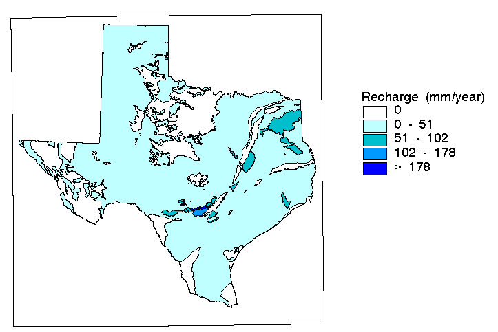
A map of DRASTIC ratings for net recharge was obtained from Dr. Samuel Atkinson at the University of North Texas. DRASTIC is a method developed by the United States Environmental Protection Agency (EPA) to assess groundwater pollution potential. Lumped recharge estimates published in TWDB Report 238 based upon zones defined by river basin and county boundaries were used to create this DRASTIC map. A simple assumption was made in the DRASTIC study to distribute this recharge over aquifer outcrop and downdip areas (Atkinson et al., 1992). Since the data obtained from Dr. Atkinson were actually DRASTIC ratings for recharge rather than explicit recharge values, these ratings were converted to recharge estimates in mm year-1 based upon Table R-2 in Atkinson et al., 1992. There are only four unique recharge rating values in the DRASTIC grid of Texas. Figure 5.8 shows that most of Texas has less than 51 mm year-1 of recharge and the highest recharge values occur in the Edward's Aquifer. Based on this recharge map, the average recharge in each watershed was calculated. Watersheds with high recharge were not considered in the development of the expected runoff function.
 Figure
5-8: Average Annual Recharge (mm/year) Based Upon DRASTIC Ratings
Figure
5-8: Average Annual Recharge (mm/year) Based Upon DRASTIC Ratings5.2.4.5 Springs
When looking at the runoff data, it became clear that springflow can dominate the runoff characteristics of watersheds in certain locations (the watershed containing Comal Springs for example). For this reason, a point coverage of springs in Texas was created using information from TWDB Report 189, "Major and Historical Springs of Texas." Springs described in Report 189 with an observed flow of at least 2 cfs at any time in history are included in this point coverage. The coverage includes spring name, maximum observed flow, and year of maximum observed flow. The reason that maximum observed flows were used rather than mean flows is that Report 189 contains limited observations for many of the springs. Maximum spring flows also serve as a conservative estimate if the question is whether or not a streamflow is significantly influenced by springflow. To try to quantify the influence of spring flow on watershed runoff characteristics, the sum of maximum spring flows within each watershed was computed, and this flow rate (cfs) was normalized by watershed area to get millimeters of springflow per year per watershed area. Use of the estimated spring flow values did not turn out to play a large role in the development of the expected runoff function because using a recharge rate criterion eliminated almost all watersheds with large spring flows from consideration.
5.3 Results and Discussion
A plot of the average runoff per unit area (mm) versus average rainfall (mm) for all delineated watersheds is shown in Figure 5.9. A trend of increasing runoff with rainfall is clear, but there are a number of outliers from the general trend. These are the points that merit further investigation. Most of the outlying points are from watersheds with significant anthropogenic influence in the form of urbanization, reservoirs, agriculture, or diversions for municipal use. A few of these outliers result from unusual hydrogeology. For example, karst formations in the Edwards Aquifer transfer significant quantities of water between watersheds delineated in this study. This results in lower than expected runoff in the watershed where recharge is occurring and higher than expected runoff in the spring fed stream of an adjacent watershed. Heavy recharge and re-emergence of this same water as springflow within a watershed may also limit evaporative losses and result in higher than expected runoff values. These observations regarding outlying points led to the hypothesis that a set of criteria could be used to define the runoff expected under conditions of minimal human influence and in the absence of large groundwater transmissions.
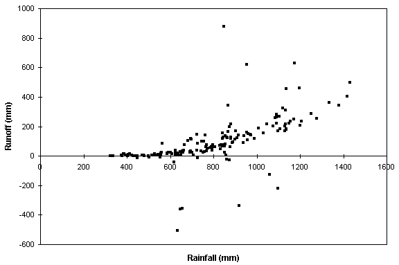
As described in the previous section, many attributes
have been compiled for each watershed. Using this set of attributes,
query tools in ArcView GIS facilitate expedient analysis of how
different criteria affect the plot of rainfall versus runoff shown
in Figure 5.9. After trying many sets of criteria, the following
set was selected as a reasonable set that produces a subset of
watersheds with a more definitive relationship between rainfall
and runoff than that seen using all 166 watersheds:
After these criteria are satisfied, two distinctive
outliers from the general trend remain. One of these points represents
data for a spring fed river in south Texas called Devil's River.
Including another criterion that limits the maximum springflow
[mm/watershed area] divided by rainfall [mm] to less than 0.03
eliminates this point. The last outlying point is for a section
of the Sulfur River in northeast Texas. The increased runoff
at this location may be due to channelization of this river by
the U.S. Army Corps of Engineers, but this is only speculation.
This point was not considered when deriving the expected runoff
function.
A function that minimizes the sum of squared errors
was fit to the remaining data points. Figure 5.10 shows this
selected set of 90 watersheds and Figure 5.11 is a plot of the
data points for these watersheds with the fitted function. The
fitted function takes the following form
P < Po (5.2)
P>=Po
where Q is runoff (mm year-1) and P is
precipitation (mm year-1). An exponential function
was fit to the data in drier areas with mean annual rainfall less
than Po ( 801 mm year-1). It turns out
that a linear function yields a better fit to the wetter watersheds
with rainfall above Po. In theory, with increasing
rainfall, one might expect the slope of the rainfall-runoff curve
to keep increasing until a value of 1 is reached, indicating that
the maximum amount of evaporation possible has been reached.
At this point, the only difference between the precipitation and
observed runoff would be the potential evaporation. The amount
of annual rainfall needed to reach this theoretical slope of 1
is certainly beyond the range of rainfall values in this data
set. Figure 5.12 is a plot of the annual runoff coefficient (runoff/rainfall)
versus rainfall based on the function of Figure 5.11.

By choice of selection criteria, the notion is that
the expected runoff function can be used to estimate natural runoff
in all areas except major groundwater recharge and discharge zones.
The map of recharge shows that 97% of the state has less than
51 mm of recharge annually, implying that estimates of natural
runoff are valid over most of the state.
Criticisms of the expected runoff curve are easy
to come by. The concept of expected runoff is artificial and
the precise form of the curve is subjective. The criteria used
in developing this curve were specifically chosen to eliminate
data points that don't fit the trend, an approach that certainly
will not please statisticians. In their defense, the criteria
used to derive the expected runoff curve are based upon real,
physical data that define the concept itself. In addition, information
from the outlying points was not discarded; this information was
used to create a map of actual runoff. The fact that data from
watersheds ranging in size from 250 to 50,000 km2 follow
the same trend, implies that the behavior represented by the expected
runoff curve is scale-independent, which is an interesting result.
Using the inference of scale-independence, the expected runoff
function was applied to the 5 km precipitation grid to create
a spatially distributed map of expected runoff. This runoff function
is not suitable for application in urban areas because data from
watersheds with considerable urbanization were not used in its
development.
5.3.2 Mapping Actual
Runoff and Evaporation
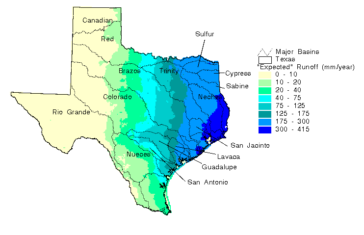
A grid of actual runoff was created on a 500 m grid by combining net runoff information at the watershed scale with expected runoff information at the 5 km grid scale. To create the actual runoff grid, an adjustment grid was created in which all cells in a given watershed were assigned the value of measured runoff per unit area less the watershed mean expected runoff, and this adjustment grid was added to the expected runoff grid (which had been resampled to a 500 m cell size). The expected runoff grid, the adjustment grid, and the actual runoff grid are shown in Figure 5.13, Figure 5.14, and Figure 5.15 respectively. The expected runoff map reflects the precipitation variation across the state. Expected runoff values range from less than 10 mm year-1 in West Texas to about 415 mm year-1 in the wettest part of East Texas.
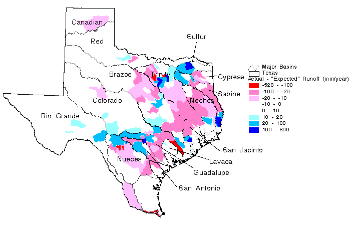
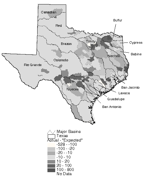
The adjustment map shown in Figure 5.14 highlights
areas with unusually large (dark blue) or small measured runoff
(dark red). Logical explanations exist for many of these "extreme"
adjustment areas. For example, the dark red areas in the lower
reaches of the Rio Grande and Colorado basins are likely caused
by large agricultural diversions in these areas. The dark red
areas in the upper portion of the Nueces basin are likely due
to large amounts of recharge to the Edward's Aquifer. Water that
recharges the Edward's Aquifer at these locations flows to the
northeast, crossing the boundaries of watersheds delineated in
this study and emerges as springflow in other locations. The
large dark blue spot in the Guadalupe basin is caused by the emergence
of Comal Springs. One drawback with using this type of runoff
map is that the effect of Comal Springs is averaged over the entire
watershed in which it emerges so it appears that a large area
is generating excess runoff when the excess runoff is primarily
due to a point discharge from groundwater. The accumulated runoff
maps described below may provide a more realistic representation
for this type of flow phenomenon. Several dark blue or dark red
areas can be seen in the Dallas area. These anomalies are likely
caused by inter-watershed transfer of water for municipal and
industrial use. Another possible explanation for the dark blue
areas near Dallas, but not for the dark red areas is that extensive
urbanization has increased the runoff coefficient.
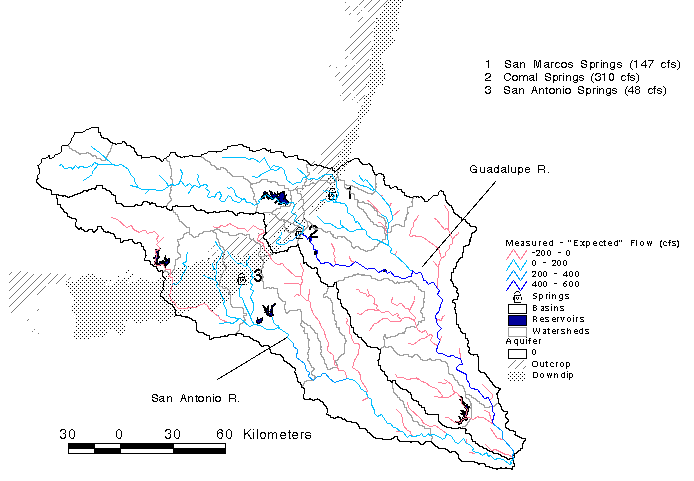
By applying a flow accumulation function to the runoff maps, the expected and actual flows were calculated at each 500 m DEM cell in Texas. Using this information, flow maps were created using line thickness and color to distinguish between minor creeks and major rivers. Figure 5.16, Figure 5.17, and Figure 5.18 are examples of these flow maps showing expected runoff, runoff adjustment, and actual runoff respectively. Flow maps of this type show statewide spatial trends such as the increased density of stream networks in East Texas, and also reveal localized phenomena attributable to large springflows and agricultural diversions. To demonstrate this further, more detailed maps for the Guadalupe and San Antonio basins are shown in Figure 5.19 and Figure 5.20. Figure 5.20 highlights the deviations from expected flow in these two basins. The influence of springs on the runoff is evident from this map. The accumulated runoff grids derived from this study could be used to attribute stream reaches with flows. An estimate of the flow is available at each 500 m DEM cell on the land surface.
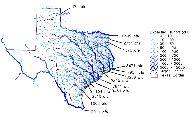
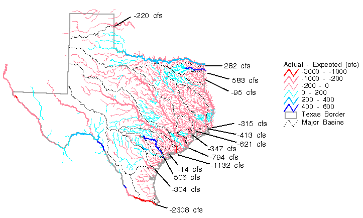
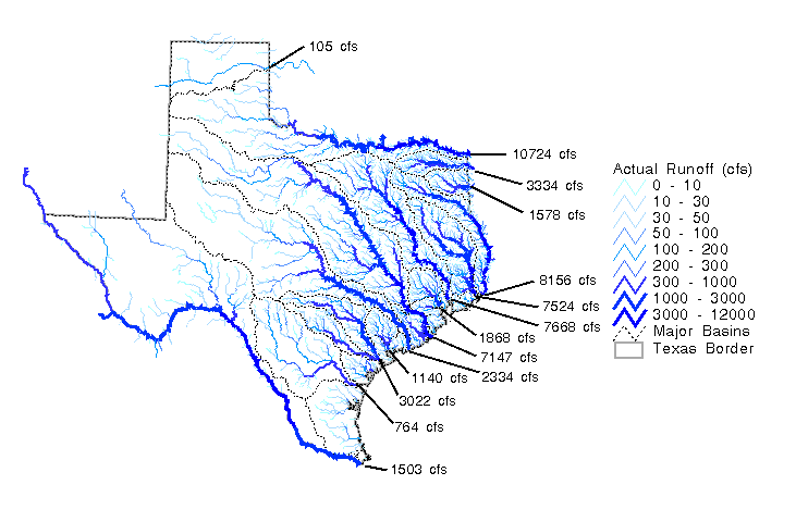
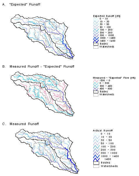
Figure
5-19: Accumulated Runoff in the San Antonio and Guadalupe Basins
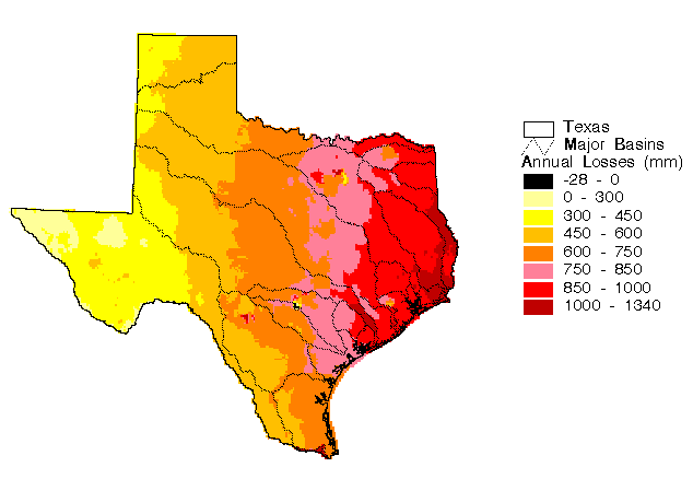
A map of losses was created by subtracting the actual runoff map from the precipitation map. Creation of this map assumes that the annual change in water storage is zero. This map of losses, shown in Figure 5.21, is equivalent to a map of actual evaporation in locations where inter-watershed transfers are negligible.
Using maps of net radiation, temperature, and expected
evaporation, a map of mean annual Bowen ratios for the State can
be computed. The Bowen ratio () is the ratio of sensible heat
flux (H) to vapor heat flux (E).
(5.3)
These flux units can be expressed in units of equivalent
depth of liquid water [L T-1]. If the ground heat
flux is assumed to be zero, then the net radiation can be approximated
as
Er = H + E (5.4)
where Er [L T-1] is
and Rn is net radiation [W m-2], lv
is latent heat of vaporization [J kg-1], and rw
is density of water [kg m-3]. Both lv an
w are functions of temperature and were estimated using
a mean annual temperature map in this case. Combining Equations
5.3 and 5.4, the Bowen ratios were estimated using
(5.5)
with E taken as expected evaporation [mm year-1]
and Er converted to the same units. Maps of mean annual
net radiation and temperature required to estimate Er
were presented in Figures 4.5 and 4.4 respectively. A map of
annual expected evaporation (precipitation - expected runoff)
is shown in Figure 5.22. The map of Bowen ratios computed from
Equation 5.5 is shown in Figure 5.23.
Figure 5-22: Expected Annual Evaporation Computed as Precipitation Minus Expected Runoff
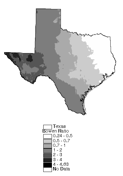
By combining the information in this Bowen ratio map with information about mean annual saturated soil moisture fraction shown in Figure 4.10, a relationship between the Bowen ratio and soil moisture fraction could be derived. This information could be used in the soil-water balance method to eliminate the need for using the potential evapotranspiration concept. At each time step, the soil moisture level is known, so the Bowen ration could be estimated from this relationship. In addition, the net radiation and temperature are known so that Equation 5.5 could be used to solve for E. This approach to estimating evaporation is attractive because it is simple and eliminates the use of the ambiguous potential evapotranspiration concept, but it needs further investigation.
Table 5.1 summarizes the annual precipitation, evaporation,
and recharge in Texas by major river basin. By virtue of the
method used to estimate evaporation, runoff equals precipitation
minus evaporation in this table. The recharge estimates in Table
5.1 are based on an independent study made by Atkinson et al.(See
Section 5.2.5.4). It is difficult to relate recharge to runoff
because recharged water may have a number of fates it may be
used to replenish groundwater storage, it may re-emerge as springflow
in a different location from where the recharge occurred, or it
may be pumped out of the ground and used consumptively by humans.
Table 5-1: Summary of Annual Hydrologic
Cycle Fluxes by River Basin
| ID | Name | Area (km2) | Precip. (mm) | Evap. (mm) | Runoff (mm) | Recharge (mm) |
| 1 | Canadian | 33262.0 | 472.5 | 471.4 | 1.1 | 24.8 |
| 2 | Red | 63641.0 | 637.9 | 594.3 | 43.6 | 18.2 |
| 3 | Brazos | 109130.3 | 735.4 | 677.1 | 58.3 | 19.5 |
| 4 | Sulfur | 9359.0 | 1153.3 | 849.2 | 304.1 | 19.8 |
| 5 | Trinity | 45721.3 | 983.1 | 833.3 | 149.8 | 21.4 |
| 6 | Colorado | 103268.5 | 609.1 | 589.0 | 20.1 | 21.4 |
| 7 | Sabine | 19538.5 | 1212.3 | 941.9 | 270.4 | 31.9 |
| 8 | Cypress | 7576.2 | 1177.4 | 927.8 | 249.6 | 56.8 |
| 9 | Neches | 25624.8 | 1208.4 | 946.2 | 262.2 | 28.5 |
| 10 | Rio Grande | 128967.7 | 396.7 | 391.3 | 5.4 | 16.7 |
| 11 | San Jacinto | 7558.2 | 1179.0 | 958.4 | 220.6 | 25.6 |
| 12 | Guadalupe | 15561.7 | 856.9 | 735.7 | 121.2 | 25.9 |
| 13 | Nueces | 43799.2 | 630.7 | 615.1 | 15.6 | 24.9 |
| 14 | San Antonio | 10946.2 | 787.6 | 713.4 | 74.2 | 55.1 |
| 15 | Lavaca | 5975.8 | 1003.5 | 833.4 | 170.1 | 25.4 |
| 16 | Coastal | 50778.5 | 1096.0 | 864.6 | 231.4 | -- |
| Texas | 680709.0 | 720.0 | 641.6 | 78.4 | 22.0 |
Table 5.2 was constructed to see whether or not the
differences between expected runoff and actual runoff are comparable
to the excess evaporation caused by reservoirs. The actual and
expected runoff values in Table 5.2 represent 30 year mean values
for 1961-1990. Since a number of reservoirs were impounded in
Texas between 1961 and 1990, the average influence of reservoirs
on runoff during this period is difficult to estimate; however,
if reservoirs were the only cause of differences between expected
runoff and actual runoff, then one might expect the values in
Column 4 of Table 5.2 to be bounded by the estimates in Columns
5 and 6. Although this condition is met for some basins, it is
not true for all basins. There are several reasons why this condition
may not be met. First, the reservoir evaporation estimates are
rough estimates based on the assumption that the average reservoir
surface area is equal to its conservation area and these estimates
involve all the assumptions used to estimating open water evaporation
using pan coefficients. Second, other factors such as agricultural
diversions may have a significant influence on the actual runoff
in some locations. Third, gross lake surface evaporation estimates
were used to compute the numbers given in Table 5.2, but it would
have made more sense to use net evaporation estimates for this
comparison. Despite these problems, there is a general trend
that basins with higher differences between expected and actual
runoff are basins with a larger amount of estimated reservoir
evaporation. Two major exceptions to this trend are the Red River
basin and Sulfur River basin. In the Red River basin, there is
a large lake, Lake Texoma, downstream of the last flow gaging
station used to create runoff maps; therefore, the actual runoff
estimate might be too high. In the Sulfur River basin, the last
flow gaging station used in the creation of runoff maps is upstream
of the only major reservoir in this basin, potentially causing
the "observed" flow map value to be too high. A channel
modification project undertaken by the U.S. Army Corps of Engineers
could be another reason for unusually high runoff observed in
the Sulfur River basin.
| Estimated Evaporation (cfs) | |||||
| "Exp." - Obs | from Reservoirs Impounded : | ||||
| Basin | (cfs) | Before 1960 | Before 1990 | ||
| Canadian | 105 | 325 | 220 | 4 | 147 |
| Red* | 10724 | 10442 | -282 | 277 | 554 |
| Sulfur** | 3334 | 2751 | -583 | 204 | 215 |
| Cypress | 1578 | 1673 | 95 | 291 | 386 |
| Sabine | 8156 | 8471 | 315 | 297 | 1585 |
| Neches | 7524 | 7937 | 413 | 102 | 990 |
| Trinity | 7668 | 8289 | 621 | 734 | 2678 |
| San Jacinto | 1868 | 2215 | 347 | 73 | 206 |
| Brazos | 7147 | 7841 | 794 | 546 | 1257 |
| Colorado | 2334 | 3466 | 1132 | 619 | 1237 |
| Lavaca | 1140 | 1154 | 14 | 0 | 75 |
| Guadalupe | 2112 | 1715 | -397 | 10 | 91 |
| San Antonio | 910 | 801 | -109 | 40 | 75 |
| Nueces | 764 | 1068 | 304 | 143 | 332 |
| Rio Grande | 1503 | 3811 | 2308 | 916 | 1462 |
| Coastal | 13158 | 12754 | -404 | 336 | 418 |
| * There is a large reservoir, Lake Texoma, downstream of the last gage. Thus, the observed | |||||
| flow might be too high for this reason. | |||||
| ** The last flow gage station is way above the reservoir in this watershed. Also, | |||||
| channel modification by the U.S. Army Corps of Engineers could be affecting runoff in this basin. | |||||
A technique for mapping mean annual runoff has been
developed and applied in the state of Texas. The procedure involved
extensive data collection and manipulation of hydrologic and geographic
data. The basic approach was to first develop an "expected"
rainfall-runoff function by plotting mean annual runoff per unit
area versus mean annual rainfall for different watersheds. The
watersheds used in the analysis were delineated from a 500 m digital
elevation model. A detailed screening process was used to identify
watersheds with limited anthropogenic influence and no large groundwater
transmissions the resulting set of 90 watersheds was used to
develop the expected runoff function. Applying the expected runoff
function to each cell in a gridded rainfall map yielded a grid
of expected runoff. To map the observed runoff, rather than the
runoff estimated from this empirical relationship, an adjustment
grid was created in which all cells in each watershed were assigned
the value of the difference between the observed runoff per unit
area and the expected runoff [mm]. After adding this adjustment
grid to the expected runoff grid, the sum of the runoff from all
cells in delineated watersheds is forced to equal the observed
flow at gaged outlets.
Many short computer programs, written mostly in Arc/Info's
script language (AML) for grid processing and ArcView's script
language (Avenue) for processing time-series data and performing
spatial analysis on vector coverages, were used in this study.
This means that making modifications to the procedure or applying
a similar procedure to another region would not be too difficult;
however, any potential user must be familiar with AML and Avenue
to modify these programs for other uses.
There are several potential uses for the runoff maps
developed in this study. A grid of actual runoff could be useful
in determining non-point source pollutant loadings in a manner
similar to that described by Saunders and Maidment (1996). The
expected runoff concept may be useful in the determination of
water rights; however, use of the specific function developed
in this study is not necessarily recommended. Water rights determination
requires an estimate of what the runoff at any location might
be in the absence of human influence. The accumulated expected
runoff grid defines how much flow is expected at each 500 m DEM
cell in Texas. The expected runoff function used in this study
serves as a useful baseline for runoff mapping and for estimating
runoff in ungaged areas; however, it is difficult to know whether
or not the watersheds used for developing the expected runoff
function are truly free from anthropogenic influence. The effects
of reservoirs and urbanization were roughly accounted for, but
other factors such as landuse changes due to farming or groundwater
pumping and surface water diversions for agriculture, municipal,
or industrial use were not explicitly accounted for in developing
the expected runoff function. The maps of observed runoff do,
however, inherently account for these other factors .
In this study, the decision was made to analyze one
time period (1961-1990) and plot data for many different spatial
locations. This was primarily a data driven decision a detailed
study had been made at Oregon State University to create a precipitation
grid for this time period. An alternative approach to developing
an annual runoff curve would be to use fewer spatial divisions
and more time divisions. For example, plotting mean runoff versus
rainfall for a few watersheds over several different years.