Homework 1 Solution

GIS in Water Resources

Fall 2010

Prepared by David R. Maidment

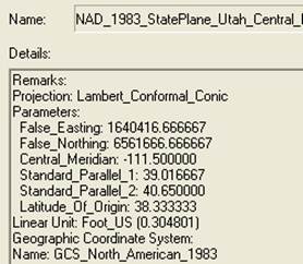
1. �Map Projection Parameters

The map below shows Utah and the display parameters of the State Plane coordinate system for the Utah Central Zone.��

���������

(a)� Sketch on the map the standard parallels, the central meridian and the latitude of origin of this projection.

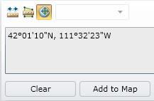I prepared the map above using ArcGIS Explorer Online.� http://explorer.arcgis.com/� The tool for locating coordinates is called Measure �and when you click on that tool, it invokes a dialog box �within which the �icon serves to select identifying a point location.��� Utah is clearly defined in latitude-longitude coordinates using meridians at 109�W and 114�W and parallels at 37�N and 42�N, making it 5� longitude x 5� latitude in area, except for a box 2� longitude x 1� latitude that is omitted in the upper right corner (I imagine the reason for this would make an interesting historical study!)

(b)� For this projection, what are the coordinates of the origin (f_o, l_o) and the corresponding (X_o, Y_o) ?

(f_o, l_o) = (38� 20� N, 111� 30� W)

(X_o, Y_o) = (1640416.666667, 6561666.666667) in meters.

Notice that the (f_o, l_o) are stated with the vertical coordinate first and the horizontal coordinate second, while the reverse is true for (X_o, Y_o)

(c)� What earth datum is used in this coordinate system?

The earth datum is GCS (Geographic Coordinate System) North American of 1983, or NAD83.

(d)�� What map projection is used in this coordinate system?

Lambert Conformal Conic

2. Locations on the Earth�

Using ArcGIS Explorer and putting in the names of Austin, Logan and Lincoln reveals the following designated locations for these cities.�� Convert these locations into decimal degrees.

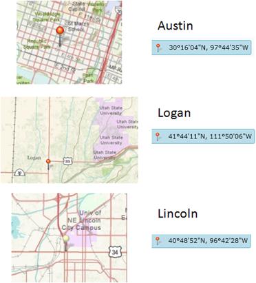
The computations are shown in the spreadsheet below.�

LatDD = LatDeg + LatMin/60 + LatSec/3600

LongDD = -(LongDeg + LongMin/60 + LongSec/3600)

So, for Austin,

LatDD = 30 + 16/60 + 4/3600 = 30.2678

LongDD = -(97+44/60 + 35/3600) = -97.7431

	LatDeg	LatMin	LatSec	LongDeg	LongMin	LongSec	LatDD	LongDD
Austin	30	16	4	97	44	35	30.2678	-97.7431
Logan	41	44	11	111	50	6	41.7364	-111.8350
Lincoln	40	48	52	96	42	28	40.8144	-96.7078

The smallest unit that distinguishes location in degrees, minutes and seconds is 1 arc second.� This corresponds to 1/3600 = 0.000278 decimal degrees.� It follows that locations in decimal degrees must be specified to at least 4 decimal places if location precision is not to be lost when conversions into decimal degrees are done.� �Also, please note that in the western hemisphere, decimal longitudes are always negative.� In other word decimal degrees are positive or negative numbers not numbers with W or N associated with them.

3.� Great Circle Distances�

The great circle distance is given by the formula

with R = 6378.137 km.

All the angles need to be in radians for formulas in Excel to work, so the above angles are converted as shown below:

	LatDD	LongDD	LatRad	LongRad
Austin	30.2678	-97.7431	0.528272	-1.70594
Logan	41.7364	-111.8350	0.728437	-1.95189
Lincoln	40.8144	-96.7078	0.712346	-1.68787

And the corresponding great earth distances are computed as follows:

	R =	6378.137
Austin-Logan		LatRad, f	LongRad, l	Distance km
	A	0.5283	-1.7059	1795.473
	B	0.7284	-1.9519
Austin-Lincoln		LatRad, f	LongRad, l	Distance km
	A	0.5283	-1.7059	1177.762
	B	0.7123	-1.6879
Logan-Lincoln		LatRad, f	LongRad, l	Distance km
	A	0.7284	-1.9519	1268.081
	B	0.7123	-1.6879

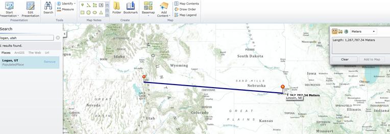
In order to check the distances between the two points, I used ArcGIS Explorer at http://explorer.arcgis.com .� I marked the three cities as described above, and then I used a measure tool to measure between pairs of marked locations.�� Here is an example for the distance between Logan and Lincoln, for which I got 1267.787 km, as compared to 1268.081 km above (a difference of 0.294 km, or 294 m), which seems reasonable given that the great circle distance we�ve computed is on a spherical earth.

The distance between Austin and Logan is 1795.183 km, and between Austin and Lincoln is 1178.257 km which are both very close to the answers given above.� Actually, it�s a bit hard to zoom into these points exactly in ArcGIS Explorer when doing this �measure� so if you could do that better, the results would probably be closer to those computed by the great circle formula.�

4.� Size of DEM cells

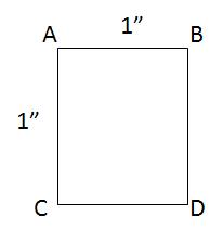
The distances AB and AC, and be computed by the formulas for distance along a parallel and a meridian, with R_e = 1378.137 km.��

There is a very slight difference in the latitude f between the top and bottom of a DEM cell, but let�s neglect that for this example, so , the area of the DEM cell is given by

The results of a spreadsheet computation of these formulas are shown below:

DEM Cells

R =

6378.137

Df, Dl =

4.848E-06

	LatRad, f	LongRad, l	Cosf	AB	AC	Area	Sqrt(Area)
Austin	0.5283	-1.7059	0.8637	26.707	30.922	825.828	28.737
Logan	0.7284	-1.9519	0.7462	23.075	30.922	713.513	26.712
Lincoln	0.7123	-1.6879	0.7568	23.403	30.922	723.662	26.901

The great circle formula given above is erroneous when applied to very short distances.� In that case, an alternative great circle formula called the �Haversine formula� can be used, as follows:

In this case, for the distance along a parallel can be given by the latitude of the location.�� Doing the calculations this way gives the following results, which are identical to the ones given above for the simple formulas for distance along a meridian and parallel.

DEM Cells	R =	6378.137	Df, Dl =	4.848E-06
	LatRad, f	LongRad, l	Cosf	AB	AC	Area	Sqrt(Area)
Austin	0.528272	-1.7059381	0.8636792	26.707	30.922	825.828	28.737
Logan	0.728437	-1.951889	0.7462155	23.075	30.922	713.513	26.712
Lincoln	0.712346	-1.6878691	0.7568303	23.403	30.922	723.662	26.901

The fact that these two results are identical can also be demonstrated mathematically.

�For distance along a parallel, �and in this case the Haversine formula reduces to

as was given earlier in the simple formula for distance along a parallel.

�For distance along a meridian, �so the Haversine formula reduces to:

as was given earlier in the simple formula for distance along a meridian.�