Prepared by Ann M. Quenzer and David R. Maidment
This exercise is intended to introduce you to land use data and introduce you to the use of soils data from the STATSGO soils coverage. The exercise is divided into six parts.
This exercise can mostly be done in ArcView but there is a Union operation near the end that uses workstation Arc/Info version 7.0. It uses a watersheds coverage Covshd10p which was derived from 3 arc-second digital elevation data for the West Austin map sheet using the procedure described in a previous exercise. It also uses the Statsgop coverage for Texas, and a clipped version of this called Soilshedp which has been clipped to conform to the watershed boundaries of Covshd10p, and a similarly clipped version of the Rf1 rivers coverage called Rf1shedp, so that you can see the association of rivers and soils in the study area. Tabular data on the soil properties are provided by the Info tables Mapunit, Comp, and Layer, which are held separately from the soil coverages in the Info directory. To save space in your file area, you will just view the Statsgop coverage for Texas from my directory alpha62:maidment:/home1/alpha62/maidment/statland/ using Arcview, rather than copying it over into your own file directory. Finally, the exercise looks at the land use in the study region and the coinciding characteristics between land use and soil type.
Make a new directory for this assignment, and change directories to this directory. The files can be found on the LRC server at: lrc/class/maidment/giswr/statland.
Download the data via anonymous ftp from ftp.crwr.utexas.edu/pub/gisclass/statland. If necessary, see instructions on how to use anonymous ftp. You need the following coverages:
and the following info files:
The total amount of file space needed for these files is 6.5MB of which 4.6MB is in the layer table. If you are short of file space, don't download the layer table immediately because it is not needed until near the end of the exercise.
These files are in export format so you will need to import them using the arc import command. For the coverages, use:
and for the info files use:
Arc: import info comp.e00 comp
Arc: import info layer.e00 layer
Arc: import info mapunit.e00 mapunit
Once you've imported the coverages and info files, you can use the Unix command rm to remove the .e00 files that you used to acquire the data. You can remove several files at once by listing them one after another with a space in between. Don't put a comma after the file names or the rm command interprets the comma as being a part of the file name:
$ rm covshd10p.e00 rf1shedp.e00 soilshedp.e00 compp.e00 layerp.e00 mapunipt.e00 auslandp.e00
or
$ rm *.e00
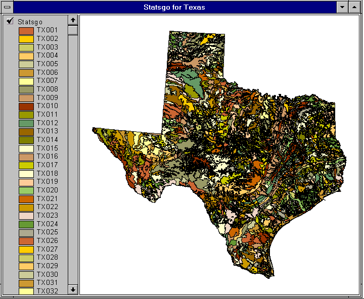
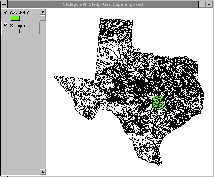
Start up Arcview. Open a new View and add the theme Statsgop which is resident in the directory home1/alpha62/maidment/statland/. If you have trouble accessing this file, I've put an export file statsgop.e00 on the anonymous ftp site and in the directory with the other files for this exercise, but beware, as this file is 17MB in size! Next, add the theme Covshd10p which is in your working directory. You can see the large number of Statsgo polygons which are needed to describe the soils of Texas (actually there are 4031 polygons in the Statsgo coverage for Texas). By superimposing the watersheds coverage on top of the soils you can see the region of analysis in Central Texas that we will work with for the remainder of the exercise.
The properties of the Statsgo coverage for Texas are:
Clearly this is an immense data base, but the large size of its polygons makes it suitable for analysis of fairly large areas which contain several Statsgo polygons. There is another database called SSURGO, still under development by US Dept of Agriculture, which details soil polygons at the component level rather than at the map unit level.
In order to create a study region that has reasonably sized files, the Statsgo coverage of Texas has been clipped using a set of watersheds Covshd10p derived for the West Austin region of Central Texas.
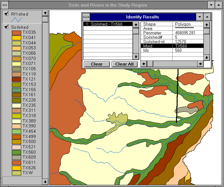
Use Edit/Delete Themes to delete the Statsgop theme. Add themes from your working directory for Soilshedp, Rf1shedp. Highlight Soilshedp and using the legend editor, use the field Muid to label the mapunits. Muid is the mapunit identification number for each unique combination soil components depicted in Statsgo.
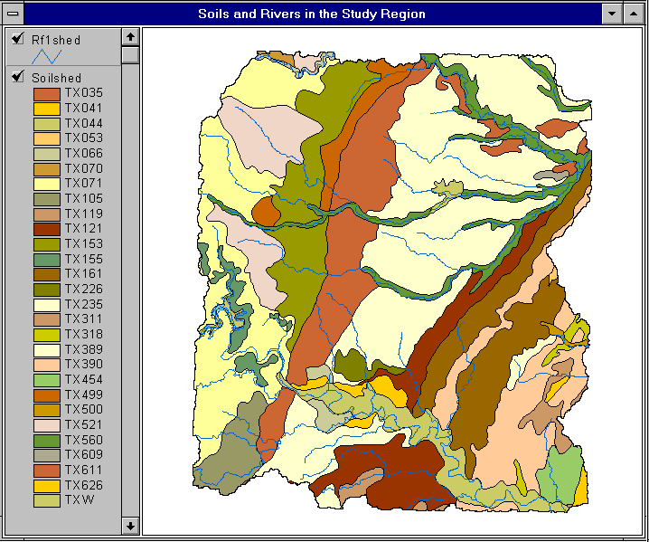
Notice how the properties of the soils are closely associated with the
location of rivers, particularly in the North-East part of the Central
Texas area that you now have displayed. Use the ![]() tool in the View window to determine the map unit that underlies many of
the rivers in that area (Mapunit Muid = Tx560). Lets take a look at the
properties of this map unit.
tool in the View window to determine the map unit that underlies many of
the rivers in that area (Mapunit Muid = Tx560). Lets take a look at the
properties of this map unit.
Click on Tables in the Project window, select Add, go to the work area where you have copied the files at the beginning of this exercise and click on the Info directory. In the left bottom box instead of "List Files of Type , select INFO files. From the Info directory, add the mapunit and comp tables to the Project. Each of these tables has a lot of fields that are not needed in this exercise so lets delete these unwanted fields from the display. Highlight the Mapunit table, and use Table/Properties to click off the check boxes Visible in all Fields except for Muid and Muname. Drag the end of the Muname field title bar to the right so you can read all of the Muname. You'll see that it is a combination of several different soil names.
Similarly, for the Comp table, click off all fields except for Muid, Seqnum, Compname, Comppct, Slopel, Slopeh, Surftex, and Hydgrp which is located near the end of the table.
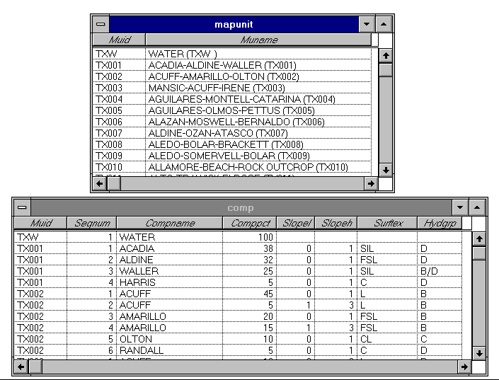
These fields represent:
Linking the Tables:
Now we are going to do something cool. The Comp table is going to be
called the Source table and the Mapunit table the Destination
table, and we are going to establish a linkage between these two tables:
Click on the "Source" table (Comp) and select the field
to be used for the linkage (Muid) by clicking on its field name
(you will see it gets depressed in the table). Click on the "Destination"
table (Mapunit), and select the key field to make the linkage (again
Muid). Go to the Tables pulldown menu and near the bottom you will see
Link you should see the blue bar at the bottom of the Arcview window,
rev up indicating that some action is taking place. Now, go to the Mapunit
table and select mapunit TX560 by clicking on it (it goes yellow). Bring
the selected feature up to the top of table display using the Uparrow button
![]() on the top line of the tool
bar. If necessary, click on the Comp table and likewise hit the
on the top line of the tool
bar. If necessary, click on the Comp table and likewise hit the ![]() button and you should see the component records for the selected mapunit
highlight at the top of the table. Pretty neat!! When you select a new
mapunit, the new components are chosen and highlighted at the top of the
component table.
button and you should see the component records for the selected mapunit
highlight at the top of the table. Pretty neat!! When you select a new
mapunit, the new components are chosen and highlighted at the top of the
component table.
This is a one-to-many relate where one record in the mapunit table is related to many records in the component table.
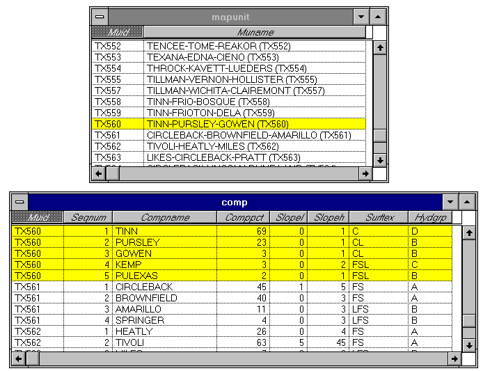
The average properties of soils in a particular map unit can be determined by using a weighted average of the component properties where the weights are equal to the percentages contained in the comppct field. For example, map unit TX560 contains soils with three surface textures: C (Clay) for component 1, CL (Clay Loam) for components 2 and 3, and FSL (Fine Sandy Loam) for components 4 and 5. The percentage of the total area in the map unit occupied by these components is 69%, 23%, 3%, 3%, and 2%, respectively. These values can be summed to give 69% surface texture Clay, 26% surface texture Clay Loam, and 5% surface texture Fine Sandy Loam.
To be turned in: Describe the TX560 soil in terms of its properties in the Mapunit and Component Tables. How many components does it have? What are their names? What percentage of the map unit does each component comprise? What is the predominant surface slope where this soil unit is found? What is the dominant soil texture? What percentage of the soil is in hydrologic soil groups A, B, C, D? Do these soil properties make sense considering where this soil is usually located?
The component properties describe the soil as a whole. Soils are usually divided into soil horizons beginning at the surface, and each horizon or layer has different physical properties. These are contained in the Layer table.
In the Project window, click on Tables and Add the Layer table to the display in the same manner that you added the mapunit and component tables. Click off all the layer properties except the following: Muid, Seqnum, Layernum, Laydepl, Laydeph, Awcl and Awch (Awc is located near the end of the table). These properties represent:
Now lets link the Layer and Comp tables together. Use the same procedure as before: click on the Layer table and highlight the Muid field. Click on the Comp Table and Highlight the Muid field. Use Table/Link to connect them. You should see a blue computational bar going along the bottom of the layer table to indicate the linking is in progress.
NOTE: Linking cannot be done while records are selected in either
Table so if you have records selected in the Comp table, unselect them
by using the ![]() icon just below
the Table menu symbol in the Table window. If you mess up and link the
wrong tables, you can use Table/Remove all Links to disconnect the
tables.
icon just below
the Table menu symbol in the Table window. If you mess up and link the
wrong tables, you can use Table/Remove all Links to disconnect the
tables.
Now lets see what we have got here. The mapunit table is linked to the
comp table and the comp table to the layer table. Click on Muid TX560 in
the mapunit table and once it is highlighted, you should see the corresponding
components and layers highlighted. Use the Uparrow ![]() icon to put the selected records at the top of the table if necessary.
Pretty cool!
icon to put the selected records at the top of the table if necessary.
Pretty cool!
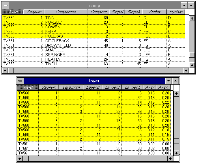
Soil Depth The total depth of the soil layer is equal to the value of laydeph for its deepest component. For example, for map unit TX560, Component 1 has depth 0 - 6 inches for layer 1 and 6 - 62 inches for layer 2 so the total depth is 62 inches (or slightly more than 5 feet) for this component.
The average depth can be found as:
Average Depth = Sum over all components of (comppct/100) * component depth
Available Water Capacity
In the layer table, the Available Water Capacity is given in dimensionless units of inches of water / inch of soil. In soil water analysis, we need to know the Water Holding Capacity of the soil, that is, the total depth of water that the soil could store within its whole vertical profile. To calculate this, we first find an average value of available water capacity for each soil layer by averaging the low and high values for that layer, (awcl + awch)/2, multiply the result by the layer thickness (laydeph - laydepl), and sum over all the layers:
Water Holding Capacity of each Component = sum over its layers of (awcl + awch)/2 * (laydeph - laydepl)
This gives a result in inches of water. For example, for mapunit TX560, Component 1 is a Tinn Clay soil having two layers, each of which has awcl = 0.15, and awch = 0.20, so the average awc = (0.15 + 0.20)/2 = 0.175. Layer 1 is 6 inches thick so its water holding capacity = 0.175 * 6 = 1.05 inches, and similarly, Layer 2 being 62 - 6 = 56 inches thick, has a water holding capacity of 56 * 0.175 = 9.80 inches of water. The total water holding capacity of the Tinn Clay component soil is 1.05 + 9.80 = 10.85 inches of water, whose storage is distributed throughout the pore spaces of the 62 inches of soil.
The average value of the water holding capacity of the soils in the TX560 map unit is found as a weighted average of the values in each component using the comppct percentages as weights:
Average Water Holding Capacity for the Map Unit = Sum over all its components of (comppct/100) * Water Holding Capacity of each Component
Computing the average water holding capacity for a map unit is a fairly involved calculation so it is probably best to transfer the data to Excel and do the calculations there. If you click on a particular Table to highlight it, you can go to the File/Export Menu option and export the selected records of that Table (the ones in yellow) into a new Table. If you choose the .dbf in the Export dialog you will produce a dBase file that can be read directly by Excel. Exporting and transferring the required records from the comp and layer tables to a spreadsheet may save you time in transcribing the data values manually.
To be turned in: For mapunit TX560, how many layers does each component have? What is the total soil depth (inches) for each layer and the average depth (inches) for the map unit? What is the total water holding capacity (inches of water) over the full soil depth for each component? What is the average water holding capacity (inches of water)for soils in this map unit?
The land use/land cover files were obtained from the Texas Natural Resource Information System's Internet site: http://www.tnris.state.tx.us/ftparea.html under the heading Land Use/Land Cover (ascii data).
These files use a Anderson Land Use Code classification system, in which major land use types are broken out into 9 categories:
The second digit distinguishes subcategories of these principal categories, e.g.
This land use classification the United States was made in the late 1970's and land use has changed in the years since then, particularly as cities have grown. But, the LULC files are still the standard land use classification of the United States taken as a whole.
More information about the land use/land cover files is contained in the GIS Hydrology Home Page.
To obtain raw data follow the report entitled Completing a Base Map for a Geographic Information System (GIS) Assessment of Nonpoint Source Pollution for the Corpus Christi Bay National Estuary Program (CCBNEP) written in December 1996, in the section Obtaining Land Use Data. This steps you through the Internet download process, importing the data, joining the files, and projecting the files.
For this exercise, only the land uses within the study region for Statsgo described earlier in the Exercise were used. The land use file that was downloaded from the TNRIS Internet site was called austina3.e00. The file was downloaded, imported, renamed to ausland, and exported for your use. Add the ausland coverage to the view. It is in your working directory.
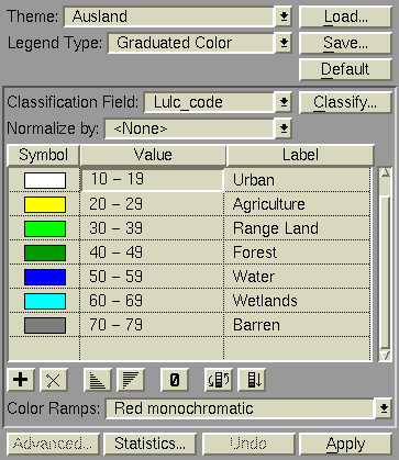
To display the individual land uses, double-click on the landuse theme symbol and, in the Legend Editor, change the Legend Type to Graduated Color and the Classification Field to lulc_code. Click on the Classify button and change the number of classes to 8. Click on the Value buttons to change the values of each category. Click on the Label buttons to change the labels of each category. Use the Fill Palette to color-code each of the symbols into land use categories.
The following color scheme works pretty well, but feel free to use your own.
| Value | Label | Symbol Color |
| 0-9 | Unknown | White |
| 10-19 | Urban | Red |
| 20-29 | Agriculture | Yellow |
| 30-39 | Range Land | Green |
| 40-49 | Forest | Dark Green |
| 50-59 | Water | Blue |
| 60-69 | Wetlands | Light Blue |
| 70-79 | Barren | Grey |
Close the Fill Palette. Click Select in the Legend Editor before closing it. Save the legend once you are finished by clicking on the Save button in the Legend Editor. The saved legend will have a .avl extension. Call the file land.avl. Now select for the landuse theme in the view and note where all the different land use categories in the basin are.
Below is what the land use coverage should look like:
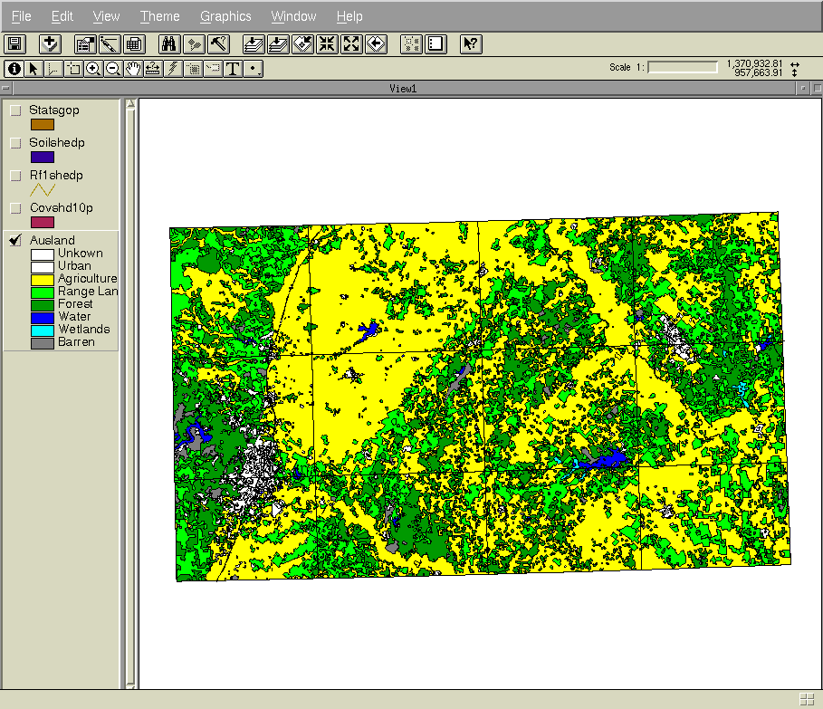
To be turned in: a map of land use in the study region
Next, we are going to make a new coverage which contains the information of both the land use and the soil data. We will do this using the Arc/Info command Union. This command will join the attribute tables from the land use and the soil coverages. It will also make a new coverage containing the joined and intersected polygon features. If you are beginning on the workstation at this point, you need the coverages soilshedp and ausland to complete the exercise. We are going to union the two coverages together, which means overlaying them so that we get new polygons, each having unique soil and land use characteristics, and we're going to inherit the attributes of the parent soil and land use coverages into the new union coverage called soilland.
$ arc
Arc: union soilshedp ausland soilland
Start up ArcView. Add the new coverage to the view and check the box to view it. Notice, how the polygons look like the land use theme and the soil theme. Click on the theme symbol to get the Legend Editor. In the legend editor, set the Legend Type to Unique. Use the field Muid to label the mapunits. Remember, Muid is the mapunit identification number for each unique combination soil components depicted in Statsgo. Click Apply, and view the new coverage. Go back to the legend editor, but this time load the land.avl legend you save earlier. When it prompts you for the field, click on the Lulc_code field. Click Apply.
You will need to look closely to find the areas that the Union command changed. It is fairly noticeable around the creeks.
To be turned in: (1) make a map of a small area of the union map which shows how a soil polygon has been cut up by being unioned with the land use coverage; (2) how many records and fields do the two original parent coverages soilshedp and ausland have? How many records and fields does the new coverage soilland have? Which of these fields are new and which are inherited from the parent coverages?
If you are using the UNIX machine, clean up the following way:
$ arc
Arc: tables
Enter Command: select mapunit
Enter Command: erase mapunit
Enter Command: select comp
Enter Command: erase comp
Enter Command: select layer
Enter Command: erase layer
Enter Command: quit
Arc: kill covshd10 all
Arc: kill soilshed all
Arc: kill rf1shed all
Arc: quit
You're done!