Regional Hydraulic Model for the City of Austin
CE 394 K.2 Surface Water Hydrology
by Esteban Azagra
Spring 1999
Table of Contents
Background
Software Requirements
Methodology
Application
Digital Elevation Model Processing
Watersheds Delineation
Hydrologic Attributes
Basin Model
Precipitation Model
Control Specifications
Flows Comparison and Model Calibration
Conclusions
Future Work
Acknowledgments
References
Geographic Information Systems (GIS) are useful tools with applications in very diverse fields of the science, some of them directly related to the water. One of the recent applications is the use of GIS in conjunction with existing computer models, not necessarily designed to work with spatial data. This term paper is intended to work in that direction, particularly in the floodplain analysis area.
Floodplain representation using computers is becoming a reality. There have been some efforts intended for the representation of water elevations (previously calculated with hydraulic models) into a Geographic Information System (GIS). This allows an easy comparison of the floodplain areas with existing buildings or other structures. More information regarding this studies can be found in Eric Tate's Homepage.
The goal of my research is the study of floodplain modeling and its representations applied to dendritic networks. In particular, this Term Project will focus on the modeling of flows. These modeled flows could be introduced into a hydraulic model in order to calculate water elevations, translating these elevations into flooded areas.
The tasks described in the preceding paragraph will be approached using the following computer programs.
HEC-HMS and HEC-RAS are two computer models, developed by the Hydrologic Engineering Center (HEC) of the United States Army Corps of Engineers, that have become a sort of standards in their respective fields. Besides, CRWR-PrePro, developed by the Center for Research in Water Resources (CRWR), has demonstrate being a very powerful tool for watershed delineation and characterization.
The Hydrologic Modeling System (HEC-HMS) is a computer program designed to simulate the surface runoff response of a river basin to precipitation, computing the streamflow hydrographs at desired locations in the river basin. In addition to unit hydrograph and hydrologic routing options, capabilities include a linear distributed-runoff transformation that can be applied with gridded rainfall data such as ‘radar’ data, a simple moisture depletion option that can be used for simulations over extended periods, and a versatile parameter optimization option. The program works around a representation of the basin as an interconnected system of hydrologic and hydraulic components that must be introduced by the user.
The River Analysis System (HEC-RAS) is a one-dimensional hydraulic model intended for calculating water surface profiles at cross-sections along a stream, for both steady and unsteady flow. The system can handle a full network of channels, a dendritic system, or a single river reach. HEC-RAS is capable of modeling subcritical, supercritical, and mixed flow regime water surface profiles. This system has became the standard computer program for modeling river and floodplain hydraulics, since the model results can be used to develop drainage designs, floodplain development restrictions, and flood insurance rates.
CRWR-PrePro is a system of Avenue scripts and controls that allows the use of hydrologic, topographic and topologic information from digital spatial data to prepare an input file that can be read by non-GIS applications, in this case HEC-HMS.
The analysis proposed for this study starts with the use of CRWR-PrePro to obtain the physical parameters describing the watersheds of the area we want to analyze. CRWR-PrePro then prepares an input file containing the hydrologic and hydraulic components of the basin that can be read by HMS.
The next step consists in running HEC-HMS in order to generate the flows we can expect after a hypothetical storm. HEC-HMS requires the input file generated by CRWR-PrePro, but also a precipitation model and time-related information for a simulation. Although this points will be detailed later, more information can be found in the exercise Introduction to HMS of the course "Surface Water Hydrology" offered in Spring 99.
Finally, the flows generated by HEC-HMS can be compared with existing values to validate the model. In this case, the existing values are those used by the City of Austin for running HEC-RAS to predict the flooding expected from hypothetical storms. As long as we use the same precipitation values, we can expect the values obtained from PrePro-HMS to be similar than the ones used by the City of Austin. If not, a model calibration will be required. More information regarding how to calibrate PrePro-HMS can be obtained somewhere else.
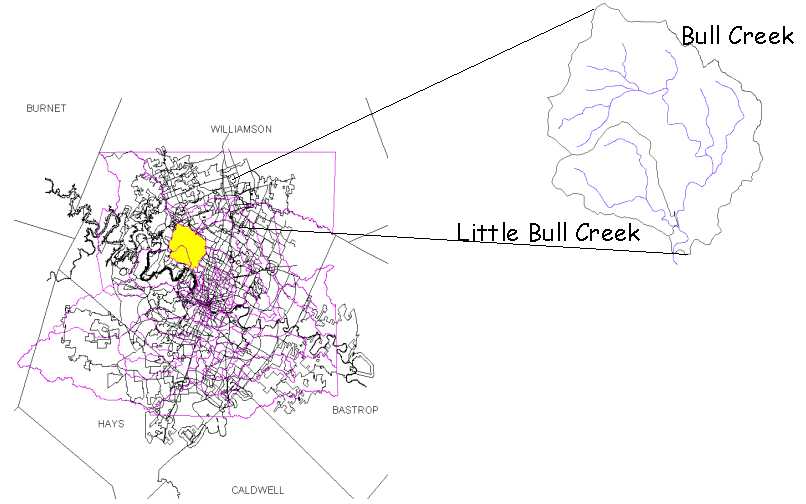
The sample area chosen for the analysis is formed by the Bull creek and Little Bull Creek watersheds, both located at the north of the City of Austin (see Figure 1). The reasons for selecting this area are:
Figure 1: Sample Area
The study required the following data:
GIS Data:
The Digital Elevation Model (DEM) necessary for delineating watersheds was provided by the City of Austin. DEMs are grids representing elevation of the terrain, and are available at several scales and levels of detail. The DEM used in the study is a 10 m grid cell.
The stream network used for the basin was the River Reach File 3 Coverage (RF3) from the United States Environment Protection Agency (EPA).
Curve numbers can be calculated from the soils characteristics included in the STATSGO database developed by the U.S. Department of Agriculture (USDA), and the Land Use/Land Cover (LULC) data developed by the United States Environment Protection Agency (EPA).
Cross sections in GIS format with the geometry of the channels were provided by the CRWR.
Non-GIS Data:
Precipitation data corresponding to hypothetical storms of different intensity can be
downloaded from a live map server accessible on the CRWR home page
http://www.crwr.utexas.edu/texas/rainfall/.
Finally, the City of Austin provided the flow values that are currently using for running HEC-RAS.
Digital Elevation Model Processing
Before running CRWR-PrePro, it was necessary to create a DEM coverage of the zone. The area was included into four separated 10 m DEM quads (corresponding to the USGS quadrangle names Austin East, Austin West, Jollyville and Pludger) and it was necessary to merge them into a single grid. This task was accomplished with the Merge Grids function of the CRWR-Raster extension.This function merges a grid with a set of grids producing a new one where the input values will take precedence in overlapping areas. Figures 2 and 3 show the four quads before and after the merging function was used.
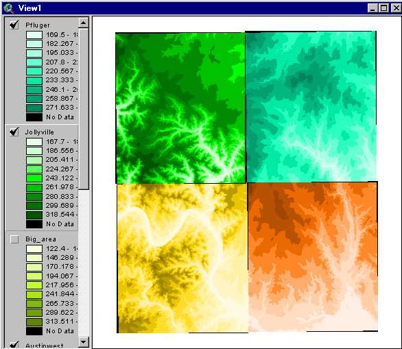
Figure 2: Austin East, Austin West, Jollyville and Pludger 10 m DEM Quads
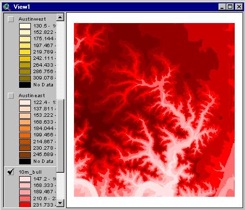
Figure 3: Merged Quads
Not all the data used was referred to the same projection and it was necessary to project all the grids in the same system. The projection system selected was the UTM Zone 14 NAD 83. Since it is not possible to reproject the orthophotos, and they are projected in UTM Zone 14 NAD 83, it will be useful for future floodplain representations to have all the maps projected in this system.
The 10 m DEM were projected in UTM Zone 14 NAD 27, instead of the desired UTM Zone 14 NAD 83. Furthermore, the altitude units were expressed in feet instead of meters. The file was projected using the ArcInfo function Project and the following projection file:
Input
Projection UTM
Zone
14
Datum
NAD27
Units
METERS
Parameters
Output
Projection UTM
Zone 14
Datum NAD83
Units
METERS
Parameters
End
Once projected, a final grid was clipped from the original reprojected DEM to reduce the size of the file. Just an area including Bull Creek and Little Bull Creek was considered. The altitude units were referred to meters using the map calculator capabilities of ArcView and multiplying every cell by 0.3048.
Once the DEM grid was ready it was possible to start delineating the subwatersheds with CRWR-PrePro. The typical sequence of work with CRWR-PrePro has already been explained somewhere else (see my GIS course Term Paper). The first step consisted in "burning in" the stream network (in this case defined by the RF3 file) into the DEM. Next was the filling of the DEM sinks and the calculation of the flow direction and flow accumulation grids. The construction of the basin stream network can be achieved by defining a threshold or minimum drainage area, or by using an existing network. In this case the second option was selected to ensure the existence of streams in those points where the channel had been previously measured and, therefore, cross-sections were available. Following, was the location of control points where the modeled flows could be compared to those used by the City of Austin. Five control points were located over five cross-sections. Next steps were the segmentation of streams into stream links and the determination of the watershed outlets. Finally, the different sub-watersheds were delineated from the calculated grids, and the result was vectorized together with the defined network. The results were a polyline shape file with streams and another one with the watersheds. Figure 4 shows the results obtained following these steps.
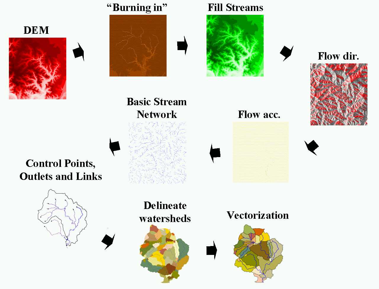
Figure 4: Watershed Delineation with CRWR-PrePro
Once the watershed delineation was completed, it was necessary to calculate the hydrologic attributes of streams and watersheds. The loss (calculation of the amount of precipitation that becomes runoff) and transform (how the excess runoff leaves the watershed) were calculated using the SCS methods. Since the calculation of the lag-time using the SCS method requires the inclusion of the average SCS curve number of the sub-basin, it was necessary to determine it as an average of the curve number values within each sub-basin polygon. A curve number grid has been calculated from the Anderson Land Use Code and the STATSGO soils data using the CRWR-PrePro. However, it was necessary to project both files from the original projections (USGS National Albers Projection in the case of STATSGO data, and Lambert in the case of LULC) into UTM. The projection was accomplished using the Projector Extension of ArcView.
With all the required information it was possible to compute the hydrologic parameters for each element and export them to HEC-HMS. It is important to point that the required information included an input file with the stream velocity and the Muskingum X. As shown later, the values of this file changed since those are the parameters that allow the calibration of the model. The last part consists on clipping out the watersheds, calculating the schematic, and generating the basin file for HMS. Figure 5 illustrates the different steps up to the generation of the basin file.
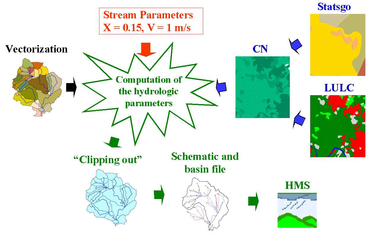
Figure 5: Hydrologic Attributes
The HEC-HMS set up involves introducing into the model information regarding the basin characteristics, precipitation and time limits. All this information is included in the Basin Model, Precipitation Model and Control Specifications.
The basin file was automatically created by CRWR-PrePro in a DSS format that can be automatically loaded into HEC-HMS. Figure 6 represents the Schematic of Bull Creek and Little Bull Creek showing the watershed and stream map and an overlay of the hydrologic elements. Notice that the number of a series of control points has been changed manually to make them coincident with the station numbers used by the City of Austin. This makes the flows comparison easier. Up to this point, the physical aspects of the model have been established.
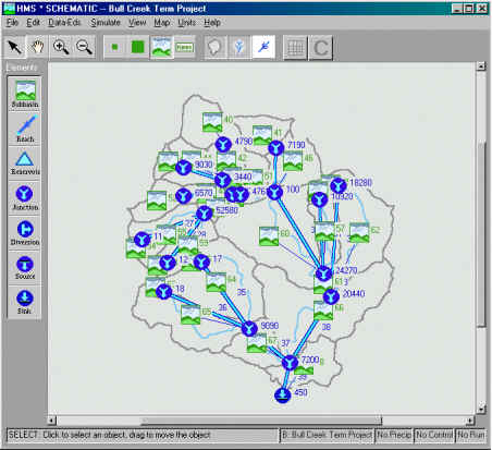
Figure 6: HMS-Schematic
Figure 7 shows information regarding the loss, transform and routing methods used in the model. As expected, the loss and transform method will be calculated using the SCS method. Depending on the length of the stream, Muskingum or Lag Time methods will be used to route the water (if the streams are too small, Muskingum is not an appropriate method and Lag Time is applied).
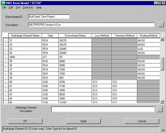
Figure 7: Basin Model
The precipitation model is the set of information required to define historical or hypothetical precipitation to be used in conjunction with a basin model. HEC-HMS allows several options for specifying hypothetical storms (frequency-based and the Corps of Engineers' Standard Project Storm) and historical precipitation (cell-based precipitation, previously determined spatially-averaged precipitation, specify gages and associated weights, or inverse distance-squared weighting in cases of missing data).
The precipitation model to be utilized in the project had to reflect the same rainfall information than the one used by the City of Austin for floodplain studies. This kind of studies are addressed using statistical analysis to determine the extreme storm rainfall expected within a given number of years. In this case, the City of Austin is using the rainfall intensities corresponding to the hypothetical storms of three hours of duration expected in the next 2, 10, 25 and 100 years.
The values used in this paper were extracted from a live map server accessible on the CRWR home page. The numbers given in this server are precipitation intensities in mm/h, so they were converted to depths in inches by multiplying by the rainfall duration and converting the resulting depth from mm to inches. The results for the storm duration used here appear on Figure 8.
3 hour duration |
2 yr design |
10 yr design |
25 yr design |
100 yr design |
||||
mm/h |
in |
mm/h |
in |
mm/h |
in |
mm/h |
in |
|
5 min |
183.5 |
0.60 |
258.7 |
0.85 |
299.3 |
0.98 |
378.0 |
1.24 |
15 min |
116.8 |
1.15 |
168.8 |
1.66 |
196.2 |
1.93 |
246.7 |
2.43 |
60 min |
49.4 |
1.95 |
73.8 |
2.91 |
86.6 |
3.41 |
109.4 |
4.31 |
120 min |
29.9 |
2.35 |
45.4 |
3.58 |
53.5 |
4.21 |
68.0 |
5.35 |
180 min |
22 |
2.60 |
33.7 |
3.98 |
39.9 |
4.71 |
51.0 |
6.02 |
Figure 8: Design Precipitation Values
Figure 9 shows an example of how the precipitation input file looks like. In this case is reflecting values corresponding to a 25 year design storm (4% chance of being equaled or exceeded in any year).
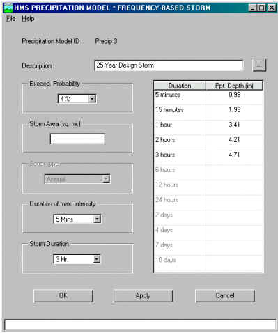
Figure 9: Precipitation Input Data for a 25 Year Storm
The last information required by HEC-HMS involves establishing the model's time limits. This information specifies the duration of the simulation in date and time, and also the interval of the calculations. A 10 minutes time interval has been selected for this study since this is the standard value used by the City of Austin. However, the model was also run using a 30 minutes interval in order to analyze the effect this parameter would have in the results. The duration selected was of two days, long enough to depict the runoff from a 3-hours storm. Figure 10 shows the Control Specification file used during the simulations.
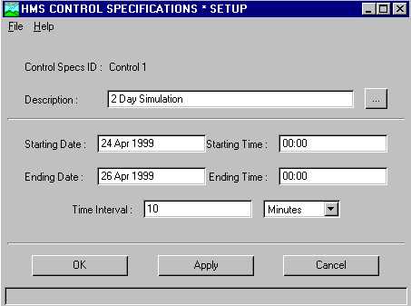
Figure 10: HEC-HMS Control Specifications
Flows Comparison and Model Calibration
After running the model for the very first time, the flow values obtained were very different from those used by the City of Austin. This suggested the model needed to be calibrated. To approach this task it was possible to change different parameters such as the flow velocity, X Muskingum, time interval or the imperviousness percentage. The last parameter would not affect the results since we were using the SCS which already accounts for the soil imperviousness through the curve number. Thus, we had the option to play with the other two parameters. The time interval should not be changed and its value should be equal to the one used by the City of Austin.
As shown in former jobs, the best parameter to be changed is the flow velocity, because its weight in the final runoff is much bigger than the corresponding to X. Therefore, the calibration was accomplished by changing the velocity and keeping the Muskingum X fixed at 0.15, which is a correct value for natural streams.
Different values of flow velocity were attempted ranging from 1.0 m/s to 1.4 m/s. It is important to notice that the flow velocity was considered equal in all the streams. This supposition is not correct and could affect the results. However, the assumption was made taking into account that the area of study is relatively flat .
Finally, as stated before, the flows were calculated for a time interval of 10 minutes (the first calculation was done using a 30 minutes time interval).
Figure 11 shows a comparison of the results obtained after running the model with the values used by the City of Austin. Control points in the table are ordered following an upstream-downstream sequence.
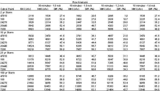
Figure 11: Flows Comparison
The differences obtained the first time the model was run were ranging between a 30 and a 60 %, depending on the storm considered and also on the point of the stream where the comparisons were made. After trying to calibrate the model, the differences obtained were still very big, ranging between a 1 % and a 30 % for a 2 year event and 1.2 m/s velocity, and between 35% and 54% for a 100 year event and the same stream velocity.
Since the differences increase as we intensify the amount of precipitation (for instance, if a 100 year storm is considered instead a 2 year storm), and considering that we are taking into account the same drainage area, there could be a discrepancy between the infiltration, transform and/or routing methods used in this study and the one used by the City of Austin.
If we analyze the SCS used in the study, we can see that the curve numbers obtained were relatively big (above 75 in any case). In fact, the method implemented in CRWR-PrePro is quite conservative. Thus, if different, the flows should have been bigger than expected.
Further calibration of the model could be attempted trying different velocities for different streams. However, the flow variations observed when different velocities were evaluated were not very large. Hence, big improvements in the results will not be achieved through this way.
As shown in the preceding table, the divergences tend to raise from the points located upstream to those located downstream, and then to reduce for the points located at the very end of the network. If the differences were always increasing as we move downstream, we could think the problem would be caused just to the infiltration, transform and/or routing methods used. However, these differences decrease at the end, indicating that some discrepancies could be due to the flow values used in HEC-RAS.
The analysis of the data provided some clues about where the problem could be. However, it is still necessary to look for a satisfactory reason to solve or al least to explain the discrepancies. Therefore, the first conclusion coming up from the paper is that further work is required to determine the causes of the differences between the modeled values and the ones used by the City of Austin. This work should focus on analyzing the methods used by the City of Austin.
However, the study has also shown that CRWR-PrePro and HEC-HMS can provide a very suitable approach for flow determinations. The method would allow the analysis of big areas with a relatively low effort and hopefully better accuracy. Furthermore, the flows resulting from HEC-HMS can be exported into a DSS format and read directly by HEC-RAS for water level determinations.
As stated in the conclusions, further work is required to compare the method followed by the City of Austin for calculating the flows they use in HEC-RAS with the one used here. This should help determine why the differences shown in this paper are so big.
GIS representation of flooded areas will be the next step. Applications as AVRAS already allow a good approach to this kind of representations, although they require the existence of a triangular irregular network (TIN) not always accessible. Exporting the water elevations from HEC-RAS would help in case no TIN were available. As shown in this paper, this kind of calculations can be done with the only requirement of having a DEM for the study area.
Finally, working with DOQ’s can help determine the centerline of the streams with more precision. As stated before, the can also help determine the structures and other buildings affected by the floodings.
Thanks to Katherine Osborne and Francisco Olivera for helping me when I needed.
Chow, V.T., Maidment, David R. and Mays, L.W. / Applied Hydrology. / New York, 1998.
Hydrologic Engineering Center. / HEC-HMS Hydrologic Modeling System, User's Manual. Version 1.0 / U.S. Army Corps of Engineers, Davis, California, 1998.
Hydrologic Engineering Center. / HEC-RAS River Analysis System, User's Manual.Version 2.2 / U.S. Army Corps of Engineers, Davis, California, 1998.
Maidment, David R. / Handbook of hydrology. / New York, 1993.
Prepared by Esteban Azagra