Introduction to AVRas
Prepared by Esteban Azagra and Franciso Olivera
Center for Research in Water Resources
September 1999
Table of Contents
Goals of the Exercise
Software and Data Requirements
Starting ArcView
Creating a TIN
AVRas Pre-processing
Preparation of Base ArcView Themes
Generation of Additional Attributes
and 3D Spatial Data
Generation of the HEC-RAS Import File
Working with HEC-RAS
AVRas Post-processing
Floodplain Representation
Cleaning Up
This exercise is intended to introduce you to computer floodplain analyses and representation using the ArcView GIS extension AVRas and the HEC-River Analysis System (HEC-RAS). The exercise covers the following concepts:
- Defining and extracting geometric data from a triangular irregular network (TIN).
- Using HEC-RAS to perform hydraulic computations to generate water surface profiles and floodway boundaries.
- Exporting HEC-RAS modeling results into ArcView to create and represent floodplain maps.
The area selected for this example is a part of the Waller Creek watershed in Austin, Texas. The exercise focuses on AVRas. If you need to get more familiar with HEC-RAS you can have a look at the exercise Introduction to HEC-RAS, prepared by Eric Tate and David Maidment.
Software and Data Requirements
The AVRas 1.2 HEC-RAS Interface extension was created by the Environmental Systems Research Institute (ESRI) and is provided for this exercise. You need to have ArcView version 3.0 or later running with the 3D Analyst extension to support surface modeling and 3D visualization.
The HEC-RAS program can be obtained from the Hydrologic Engineering Center's home page at http://www.wrc-hec.usace.army.mil/. A user's manual is also available at this location. The program runs on Windows 95/98, NT and Unix platforms. This exercise requires that you have HEC-RAS version 2.1 running.
The data files used in the exercise consist of ArcView shapefiles, AVRas extension files, and "GENERATE" files for the digital terrain model. The following files are stored in avras.zip:
- avras.avx - corresponds to the AVRas extension and should be located in the esri/av_gis30/arcview/ext32/ folder of your computer.
- avras.cnt, avras.gid, avras.hlp -help files for AVRas. They must be in the esri/av_gis30/arcview/help/ folder.
- bank.dbf, bank.shp, bank.shx -shapefile of bank locations.
- build.dbf, build.sbn, build.sbx, build.shp, build.shx -shapefile for the buildings.
- cross.dbf, cross.shp, cross.shx -shapefile of cross-sections.
- flow.dbf, flow.sbn, flow.sbx, flow.shp, flow.shx -shapefile of flow boundaries.
- hardl.lin, massp.pnt, softl.lin -GENERATE files used to create the TIN.
- terrain.avl -theme color schemes.
- transport.dbf, transport.sbn, transport.sbx, transport.shp, transport.shx -shapefile for the roads and streets.
Select a working directory on your computer and download these files into it (except those corresponding to the AVRas extension).
Before you go on, you need to set the working directory. From Project menu, choose Properties. Type the name of your working directory (where you downloaded/copied the files) in the Project Properties… dialog box and click OK. You can create a temp folder under your working directory. Save the Untitled Project as avras.apr in the working directory.
Select the File/Extensions… menu option and check the 3D Analyst and AVRas 1.2 HEC-RAS Interface extensions from the Extensions window. Click OK and the extensions will be loaded.
AVRas extracts terrain information stored in TINs and generates a geometry file that can be read by HEC-RAS. TINs can be created from points, polygons, and lines stored in different formats. In this exercise we will use GENERATE input files - ASCII files containing x, y coordinates and z values for point or breakline features- to create our TIN.
Double-click on the Views icon in the Project window to open a new view. You can change the name of the view if you want and call it "Input Data".
With the new view active, import the data stored in the GENERATE files using File/Import Data Source... and choosing the 3D Generate File from the menu. Notice that ArcView allows you to import data stored in different formats. Click OK to confirm your selection.
Choose Points as the type of input generate file you are importing and click OK. Select the file massp.pnt from your working directory and click OK again. From the new window, type massp.shp as the name of the output shapefile. You can click OK one more time to start importing the file. Select Yes to add the shapefile generated to the View.
Repeat these steps two more times to import the information corresponding to the soft and hard breaklines. Select Lines as the type of input generate file. Choose the softl.lin and hardl.lin files when asked for the name of these files and name the shapefiles created softl.shp and hardl.shp respectively. You should be able to see something similar to this:
The next step is the generation of the TIN. Select the three themes you just created, go to Surface menu and the click on Create TIN from Features.... The Create new TIN window will appear and you will have to specify the following fields for each active theme:
- The Class field specifies which type of feature is stored in the shapefile. This information is read from the shapefile and you do not have to type any value here. The value PointZ will appear if you select the Massp.shp file. For the other two files - Shoftl.shp and Hardl.shp- the value will be PolyLineZ.
- The Height source field specifies what field is used to provide height values for the theme. The value <none can be used for representing features like area boundaries. In this case, the value Shape is automatically prompted for the three files. PointZ and PolyLineZ are 3D features and their height can be determined from their shape.
- The Input as field specifies what surface feature type the theme will be added as. Check that the value selected for Massp.shp is Mass Points, and the ones corresponding to Softl.shp and Hardl.shp are Soft Breaklines and Hard Breaklines respectively.
- The Value field specifies what field - if any- is used to provide values for nodes or triangles. If the output type is mass point, the values will be assigned to nodes. If the output type is polygonal, the values will be assigned to triangles. Values are stored with the TIN data model and can be used later for display, query, and modeling purposes. For this exercise we will not assign any value to the TIN.
Click OK and type "wallertin" when asked for the TIN name. After some calculations, the TIN theme will be added to your view. Click the check box to display it. The default color scheme is not ideal for observing the TIN. Double click on the TIN’s legend bar to open the TIN legend editor. First click off the check box next to Lines and then click the Edit button in the Faces part of the window to open the regular legend editor. Click on the Load button and choose terrain.avl from your working directory. Click OK twice in the Load Legend windows and Apply in the legend editor. Your TIN should look like this:
We no longer need the themes massp.shp, softl.shp and hardl.shp, so you may delete them from the window. It would be a good idea to save your project at this point of the exercise.
The goal of this part of the exercise is to develop the basic spatial data required to generate the HEC-RAS Geometry Import File with the 3D stream network and the 3D cross section definition. The process is divided in three steps:
- Preparation of ArcView themes defining the stream centerline, cross-sections, stream banks and flow path lines.
- Use of AVRas functions to develop additional attributes required by HEC-RAS and to generate 3D spatial data.
- Generation of the HEC-RAS Import File.
Preparation of Base ArcView Themes
The shapefiles required for the definition of the stream centerline, cross-sections, stream banks, and flow path lines are provided for this exercise. However, it is important to show you how to create these files. Remember that you DO NOT have to do this part to complete this exercise.
First you will need a Digital Orthophoto Quadrangle (DOQ) or another type of
visual data source to identify the centerline, banks, and flow paths. You will
have to create a new theme for each of the required data sets. For each one,
with the view window active, select New Theme... from the View menu.
Choose a Line type theme and click OK. After choosing a name for your
new theme, you can start delineating by clicking the ![]() button. Select Theme/Stop
Editing as soon as you finish digitizing and click Yes to save the
file. There are some important rules that you have to follow during the
digitizing process to ensure the correct operation of the AVRas functions:
button. Select Theme/Stop
Editing as soon as you finish digitizing and click Yes to save the
file. There are some important rules that you have to follow during the
digitizing process to ensure the correct operation of the AVRas functions:
- All the lines must be snapped at common nodes and each individual polyline should consist of only one part. Use the snapping capabilities of ArcView to ensure this continuity.
- Stream segments and cross-sections have to be identified following certain rules. The attribute tables corresponding to each of the shapefiles have to follow the same format as the ones included in this exercise.
- Stream centerlines, flow paths and bank lines have to be pointing downstream and cannot intersect.
- Cross-sections must be digitized from the left bank to the right bank (facing downstream). Each cross-section must cross the stream centerline exactly once, the bank lines exactly twice, and the flow paths exactly three times. They cannot intersect each other. They can be entered without a specific order; only the location of the cross-sections is important.
We are going to carry on with the exercise at this point. Lets start loading the shapefiles corresponding to the centerline, flowpaths, banks, and cross-sections.
With the view window active, select Add Theme... from the View menu. Choose centerline.shp from your working directory and click OK. If you click off the check box of the TIN your view should look like this:
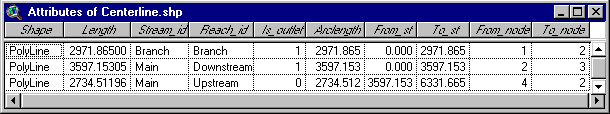
The centerline theme contains the lines defining the stream network that
will be reconstructed as the river schematic within RAS. As we already
indicated, the stream centerlines have to be oriented towards the downstream
direction and snapped at nodes. Click the ![]() button to see what the Attributes
table of Centerline.shp looks like.
button to see what the Attributes
table of Centerline.shp looks like.
- The Stream_id and Reach_id fields are character fields included to identify the streams and reaches names. These values were entered manually for each shape in the theme when it was created. Notice that one stream is made of one or more reaches.
- The is_Outlet numeric field helps identify if the end of a given reach is an outlet or not: "0" means that there is no outlet and "1" indicates an outlet at the end of the reach. Again, the values were typed manually for each shape in the theme.
Close the table and repeat the previous process to open the banks.shp theme from your working directory. If you click off the centerline your view must be like this:
The banks theme contains lines depicting the two banks of the main stream. The location of the banks along each cross-section will be calculated and stored in the cross-section attribute table. The bank lines do not have any significant orientation or specific attributes in the attributes table.
Open the shapefiles Flow.shp and Cross.shp following the same procedure. If you click on these new themes and click off the banks theme your view will be like this:
Notice that you have three flow paths for each reach. These lines are used
to calculate the reach lengths. Once more, the lines have to be oriented
towards downstream direction and lines representing the same flow path should
be snapped at common nodes. Click the ![]() button with the Flow.shp theme
selected to see its Attributes table.
button with the Flow.shp theme
selected to see its Attributes table.
- The Linetype character field is used to define the location of the lines compared to the centerline: "L" corresponds to the left overbank; "M" refers to the main stream (coincident with the stream centerline); and "R" identifies the right overbank. These values were entered manually.
The cross-sections theme contains the lines defining the cross-sections required by HEC-RAS. As in the case of the bank lines, the attributes table does not require the introduction of any particular value (we will derive some using AVRas).
Generation of Additional Attributes and 3D Spatial Data
In this part of the exercise we will make use of the base data we created to develop additional attributes required by HEC-RAS and to generate 3D features with z values to define elevations.
Lets start with the generation of the additional attributes. Select Theme Setup… from the AV-Ras menu and fill in the window as shown in the graphic. Click OK to confirm the values.
Select Centerline Topology from the AV-Ras menu. You should
see a message indicating that the process was completed successfully. Click OK
to close the window. You can compute the stream and reaches distances using the
function Length/Station Comp. in the AVRas_Util menu. Click OK
to close the message (indicating the success of the calculations) and click
the ![]() button with the Centerline.shp theme selected to see its new Attributes
table. It should look like this:
button with the Centerline.shp theme selected to see its new Attributes
table. It should look like this:
You can see the new fields added to the table:
- The From_st and To_st numeric fields indicate the name of the station up and downstream within a reach. The name matches the cumulative distance from the origin of the corresponding stream.
- The From_node and To_node numeric fields show the unique ID for the upstream and downstream node of the reach.
- The Arc_Length numeric field indicates the length of each reach in theme units (in this case feet).
Close the table and select Centerline Z Extract from the AV-Ras menu. Type "Centerline3D.shp" when asked for the theme name and click OK to confirm. Click OK to close the message confirming that the process was completed successfully. A 3D shape file has been added to the view.
The next step is the addition of new attributes to the cross-sections shapefile. Select Basic CS Attributing from the AV-Ras menu. A message will indicate that each cross-section now has a Stream_ID and a Reach_ID assigned. Click OK to close the window and select Station CS Attributing from the AV-Ras menu. Again, a message will indicate that each cross-section now has a station number assigned. Click OK one more time to close the window. To compute the cross-section bank percentages (% distance of total cross-section length) you have to select Bank CS Attributing from the AV-Ras menu. Close the window by clicking OK. We are almost done with the calculation of attributes. We just need to determine the downstream cross-section distance along the main channel, left, and right flow paths. Select Distance CS Attributing from the AV-Ras menu and click OK to close the window (with the message indicating the end of the computation). The final attribute table for the cross-section looks like this:
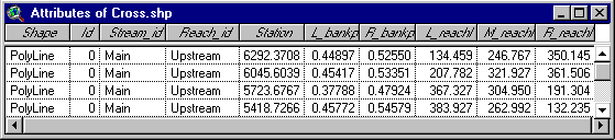
The identification and meaning of the new fields is straightforward.
Close the table and select AV-Ras/CS Z Extract. Type "Cross3D.shp" when asked for the name of the theme and click OK to confirm. Click OK to close the message confirming that the process was completed successfully. A new 3D shape file has been added to the view. This is probably a good moment to save your work.
Generation of the HEC-RAS Import File
The Generation of the HEC-RAS Import File is the last step of the AVRAs Pre-processing. The idea is to create a HEC-RAS input file in RAS GIS Import format with the terrain elevation extracted from the TIN and included in the 3D stream centerline and 3D cross-sections themes as z values.
Click the ![]() button and ignore the warning message by clicking OK.
Select ENGLISH units when asked and click OK to confirm your
selection. Once the generation of the RAS GIS Input file header is completed,
you can click OK again and wait for the processing of the information
regarding the centerline. Click OK to start processing the
cross-sections information and click OK one more time at the end of the
process. Save your project and close ArcView. You can use Windows Explorer to
check that a file called waller.geo has been created in your working
directory.
button and ignore the warning message by clicking OK.
Select ENGLISH units when asked and click OK to confirm your
selection. Once the generation of the RAS GIS Input file header is completed,
you can click OK again and wait for the processing of the information
regarding the centerline. Click OK to start processing the
cross-sections information and click OK one more time at the end of the
process. Save your project and close ArcView. You can use Windows Explorer to
check that a file called waller.geo has been created in your working
directory.
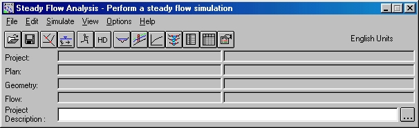
The first time you start HEC-RAS you will see the main project window, which looks like this:
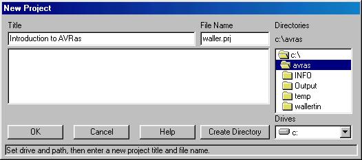
Go to File/New Project to define a new project. Select your working directory and then type the title "Introduction to AVRas" and the file name for the project "Waller.prj". Click OK and a window will open confirming the information you just entered. Click OK one more time and check that the Project line in the main project window is now filled with information.
We can keep on going and import the geometric data stored in RAS GIS Import format that we created with AVRas. Select Edit/Geometric Data… from the main project window and File/Import Geometry Data/GIS Format… from the Geometric Data window. Choose the file waller.geo from your AVRas working directory and click OK. The resulting view shows the schematic of Waller Creek.
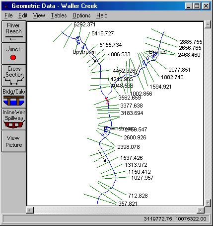
You can edit this geometric data if you want. The tick marks and corresponding numbers denote cross-sections. You can edit these cross-sections and plot their profiles. Notice that special cross-section types, such as bridges or culverts, need to be manually entered.
We are going to set the values for the Manning coefficients. Select Tables/Manning’s n or k values from the Geometric Data window. The Edit Manning’s n or k Values window will appear. First choose the value (All Rivers) in the River drop box. Click on the n#1 box to select the entire column and click the Set Values button. Type a value of "0.04" and click OK. Repeat this process for the n#2 column entering a value of "0.03" for n, and also for the n#3 column choosing a value of "0.04". The window should look like this:
Click OK to confirm the values. Select File/Save Geometry Data and then File/Exit Geometry Data Editor. You will be back to the main project window, which will have some new information in the Geometry line.
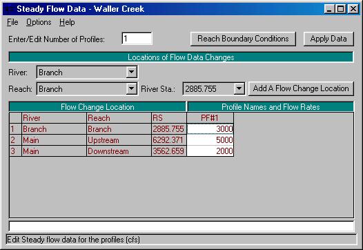
The next step is the definition of the Flow Data. For this project we will assume some hypothetical flow values.
Select Edit/Steady Flow Data… to start introducing flow values and fill the PF1 column as shown below.
Click on the Reach Boundary Conditions button. The new window is used to set the water surface elevation boundary conditions. We will use the normal depth option. Click in the last cell of the Downstream column an then click on the Normal Depth button. Set the energy slope at the boundary to "0.001" and click OK to confirm this value.
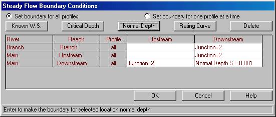
Click OK again to leave this window. Apply these flow data with the Apply Data button and save the information in your working directory selecting File/Save Flow Data. You can type a title for the data, the file name Waller.f* is given. Select File/Exit Flow Data Editor to return to the main project window. Notice the information added to the Flow line.
Now that the geometry and flow data have been set we can execute the model. Select Simulate/Steady Flow Analysis… from the project window and define a new plan - to specify the files to be used in the simulation- with File/New Plan. You will be subsequently asked to provide a plan title (i.e. Hypothetical flow conditions) and a 12 character short identifier. Click OK twice to confirm your selections.
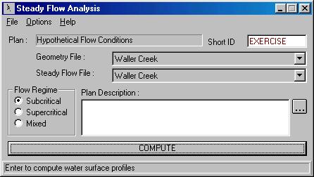
Ensure that the Flow Regime radio button is set to Subcritical and click the COMPUTE button. This starts a FORTRAN program called SNET, which carries out all the calculations. A DOS window with a message indicating the end of the process will appear when the computations are completed. Close the DOS window by clicking the X in the upper right corner. Select File/Exit to return to the main window and start exporting the results of the analysis into GIS.
Before exporting the results, you may want to have a look at the water profiles, cross-sections and perspective plots like the one shown below.
To export the data select File/Export GIS Data… from the main window.
Select the export file name as "waller.gis" and be sure you
that you save it in your working directory (or somewhere else where you can
find it). Click OK to confirm the file name and click the Export Data
button on the new window. The process is completed. You can now close HEC-RAS
saving your changes.
With the water surface elevations calculated and exported by HEC-RAS we can continue with last part of the exercise. All themes developed during the post-processing are based on the content of the RAS GIS output file and the TIN. AVRas will create a TIN with the water surface elevations and will compare this TIN with the terrain TIN to define the flooded areas. Finally, the flooded areas will be converted into a polygon theme and form the resulting flood plain theme.
Start ArcView and open the avras.apr project you saved at the end of the pre-processing phase. Select Theme Setup… from the Ras-AV menu and fill the window as shown below:
Click OK twice to confirm your selections and to dismiss the window.
Select CS/BP Generation from the Ras-AV menu to generate a 2D cross-section theme and a bounding polygon theme, based on the RAS GIS Export File you just created. A window will tell you that the process has been completed. Close it by clicking OK. A new view has been created with the name you selected for the output directory and three themes in it. It should be similar to this:
Click the![]() button with the OutputCS.shp theme selected to see its attributes
table. It should look like this one:
button with the OutputCS.shp theme selected to see its attributes
table. It should look like this one:
Each cross-section now contains the stream and reach identifiers, station number, a field indicating if the corresponding cross-section was interpolated by HEC-RAS or not, and fields (in this case just one) specifying the water surface elevation in feet as was defined in the RAS GIS Export File.
The Bppf_1.shp bounding polygon theme contains polygons depicting the bounding polygons of the RAS analyses. Polygons generated for different water surface profiles would be stored in a separate bounding polygon themes.
Select WS TIN Generation from the Ras-AV menu to create a TIN representing the water surface elevations. Click OK to close the information window. A new theme for the water surface TIN should be in your view.
We are almost done. AVRas is now going to compare the water elevation with the terrain to define the flooded areas, and will convert these areas into a polygon theme.
Select Floodplain Delineation from the Ras-AV menu. Close the information window by clicking OK and change the legend of the Fppf_1.shp theme to make it look like water. You should be able to see something like this:
Lets do a final effort to improve the floodplain representation. First, we
have to get rid of the two "islands" of water formed close to the
junction with the main stream. Select Theme/Start Editing with the Fppf_1.shp
theme selected to start editing the theme. Click the ![]() buttton and select the
two polygons you want to delete. Select Edit/Delete Features and stop
editing by selecting Theme/Stop Editing. Confirm your changes.
buttton and select the
two polygons you want to delete. Select Edit/Delete Features and stop
editing by selecting Theme/Stop Editing. Confirm your changes.
Finnaly, click the ![]() button to add the buildings.shp and transport.shp
themes. We can use these two themes as a background to identify which
facilities are affected by the water. The result should look like this:
button to add the buildings.shp and transport.shp
themes. We can use these two themes as a background to identify which
facilities are affected by the water. The result should look like this:
You can try and use the 3D Analyst capabilities to create a 3D Scene of the flooded area. You can play with the height of the buildings and use your imagination to create something like this!
Welcome to the end of what I hope gave you more of an insight of how ArcView and HEC-RAS can work together to produce floodplain maps. Remember that the key point for accurate results is to have a detailed terrain model. Go ahead and close ArcView, saving your project.