|
|
Research Work |
|
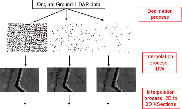
The overall objective of this project is to determine the optimal post spacing of LIDAR-derived triangulated irregular networks (TINs) and digital elevation models (DEMs) that is required to achieve different levels of accuracy in the prediction of flood risk using hydrologic and hydraulic (H&H) models. High spatial resolution LIDAR data will be used to generate a variety of TINs and DEMs for test and evaluation. These data will be entered as input to FEMA-approved H&H models at varying resolutions to determine the models' sensitivity to these changes. Research for this project is being conducted in two locations -- North Carolina and the Brownsville, TX - Matamoros, Mexico region. The results of this project will be of interest and value to state and local governments as they decide whether to use LIDAR data and at which posting density they should collect the data to predict flood risk at acceptable levels of accuracy. If they can use a more coarse posting density to accurately predict flooding over the types of terrain in their area, then this could result in huge cost savings as they update their FEMA Flood Insurance Rate Maps (FIRMs). It will also aid FEMA in their development of requirements for floodplain mapping using LIDAR.
Advanced LIDAR Technology, Inc. provides airborne laser mapping services. LIDAR stands for LIght Detection And Ranging. Basically its like radar, except with laser light instead of sound. Flown from a helicopter or fixed wing aircraft, eye safe laser pulses are sent to the ground and their reflections back are recorded. Accurate distances are then calculated to the points on the ground and therefore elevations can be determined for not only the ground surface but the buildings, roads, vegetation and even something as small as powerlines. These elevations are combined with digital aerial photography to produce a digital elevation model of the earth. As the output is digital many different final display products are possible. LIDAR mapping can benefit many different industries including:
The Center for Space Research in Austin is currently developing some algorithms to classify the LIDAR data. The objective of this classification is to separate the data into three types: - The ground For more information about this subject, please consult the website of Amy Neuenschwander's and the website of the CSR. Other data can also be derived. The Bureau of Economic geology in Austin has done an Analysis of Land Cover/Land Use.
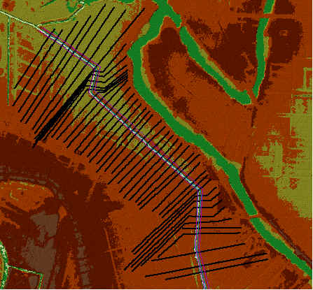
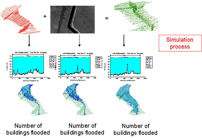
The area of interest is the North Main Drain located in Brownsville (Texas). The region is characterized by very high frequency floods. The steady state flood simulations have been made with a 1D model developed by the US Army Corp. (HEC RAS). Basically the model computes the height and the flow of the water at each Cross-Section and the flow is assumed to be perpendicular to the Cross-Sections. The simulations are calibrated for the 25-year flood based on a survey made by the engineers in Brownsville. The Manning's n coefficients have been derived from the land use data obtained with a satellite image (Land Sat).
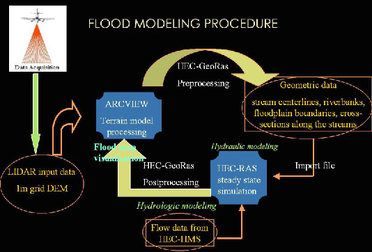
48 Cross-Sections of the North Main Drain Technically the geometric data of the model (3-D Cross-Sections) have been developed in ArcGIS using the preprocessor HEC GeoRas. These data have then been exported into HEC RAS in order to run the simulation. The results have then been re-exported into ArcGIS. The whole process can be summarized as follow:
Three different output have been studied: -The flood plain polygon
Flood plain Water Surface Elevation
The objective is to understand the influence of the density of the LIDAR data on the flood plain delineation. I have also studied the influence of the density of the LIDAR data on the delineation of the watersheds. Here is a brief description of the different steps required to do the sensitivity analysis.
Since the number of simulations required to have a good understanding of the phenomenon is high, and given the fact that a simulation is time consuming and that the probability to make an error during all these process, I had the idea to automate these operation by using the model builder. The idea is: -
To run the simulations without human intervention to avoid errors and save
time. On the model builder, the tools (actions or process) are materialized by a rectangle and the bubbles are the inputs or the outputs. The following graph represents the beginning of the chain of actions which allows to go from LIDAR data to flood map without human intervention (for more information about the model builder look at Tim Whiteaker's homepage.).
The originality of my work is that I used the Model Builder for the sensitivity analysis, which means that I figured out how to call a model with a VBScript and run it automatically with different sets of parameters by looping. For more details about lopping using the Model Builder click on the following link: looping with Model Builder.
A method has been defined to compare surfaces: it was necessary to study the evolution of the flood polygons or the watershed as density of LIDAR data decreases. The following schema presents the idea: Area A is the polygon of reference obtained with the highest density of points. Area B is a polygon obtained with a lower density.
The 2 year-flood, the 5 year-flood and the 25 year-flood event have been studied. For each of these events, 70 simulations have been made with different densities of points and the flood polygons and the number of buildings flooded have been of interest. 2-year Flood event:
5-year Flood event:
25-year Flood event (only 26 simulations have been made because when the density decreases to much the extend of the flood polygon is limited by the extend of the cross sections: larger cross-sections should have been used):
Three conclusions can be drawn from these simulations:
When a "dam" appears at a cross-section, the flow and the height computed are completely wrong and the LIDAR data with this density cannot be used anymore: the flood polygons computed as well as the number of buildings flooded are unusable.
|
|||
 |
|
||