
There are several reasons why this project was chosen and why it holds particular relevance to this area. The topic of air quality is not always the first on anyone's mind when it comes to environmental applications for a GIS system. In fact, the great majority of the time, GIS is used for a water or groundwater analysis. Dr. Allen and Dr. Kinney of the University of Texas' Program in Air Resources Engineering inspired the project by mentioning how a GIS might be useful in studying the effects on air quality of increased truck traffic on IH 35 due to NAFTA. Although this was the initial objective, a lot of groundwork needed to be done before any study of that kind could be initiated. This term project focuses on that work. This term project is the initial database development for an emissions estimate model using GIS.
For the study, the two main emissions that are of concern are volatile organic compounds (VOCs) and nitrogen oxides (NOx). These are of particular importance when it comes to air pollution because they both contribute to the production of ozone. Ozone is not emitted directly into the air but is formed through chemical reactions between natural and man-made emissions of VOCs and NOx in the presence of sunlight. These gaseous compounds mix in the ambient air, and when they interact with sunlight, ozone is formed. Sources of these pollutants include automobiles, gas-powered motors, refineries, chemical manufacturing plants, solvents used in dry cleaners and paint shops, and wherever natural gas, gasoline, diesel fuel, kerosene or oil are combusted.
It has been estimated that as much as 30 to 45 percent of the VOC emissions in the Austin area comes from on-road emissions. Although Austin is currently classified as an attainment city (city that has not exceeded the EPA national regulated standard for more than three times in any three years), the city has peaked at or very near that amount several times. (1985 levels exceeded the standard twice).
One of the concerns is that any increase in truck traffic on IH 35 will detrimentally affect Austin's air quality because the only route that is available for the trip from Laredo to Dallas/Ft. Worth is through the center of Austin.
The first step in this project was to determine the method that
was to be used for converting the obtainable interstate 35 traffic
data into an amount of pollution that was being introduced into
the atmosphere. After talking to several people in the University
of Texas Program in Air Resources Engineering (UTPARE), it was
determined that the best way to accomplish this would be to use the EPA vehicle emissions model Mobile 5a. This program is free to the public and can be downloaded from the EPA's Vehicle and Engine Emission Modeling Software page.
The Mobile programs were developed for use in determining the on road source emissions for an urban setting. However they should be able to produce a reasonable estimate for the amount of emissions that vehicles emit for highways provided the inputs to the program are precise enough. Mobile has many different versions with the latest available being Mobile 5b (the second set of modifications to Mobile 5). In this project Mobile 5a was used because of its availability and because it was the version that members of the UTPARE were most familiar with.
The program was first downloaded off the net at the EPA site. Example inputs and an instruction manual can also be found here. The files were "zipped"; and had to be opened with PKUNZIP. This is also available to the public and can be found at PKWare, Inc. as well as many other sites.
After obtaining the model, the next step was to learn what the inputs and outputs consisted of and how to use them. To run Mobile an input file that is formatted correctly is required. An example of one of my input files can be found here.
EXAMPLE INPUT FILE: 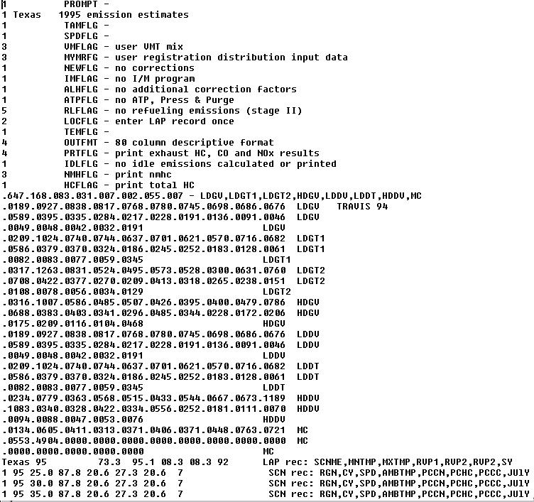
EXAMPLE OUTPUT FILE: ![]()
OK, so what does all this mean? To understand the input and output files better please go to Deciphering Mobile 5a in the appendix.
There were 4 main inputs for the Mobile 5a program that had to be obtained to produce reasonable estimates of IH-35's pollution contribution.
1) VMT mix (eight class breakdown of traffic)
2) Average Speed
3) Fleet Distribution (age distribution of vehicles)
Once the model ran for the region of interest, the average effluent
loading for each vehicle had to be multiplied by the
total vehicle density for that region. This gave the total contaminant
contribution for that region of IH 35. Or more simply put:
Load(total) = Load/Vehicle * Vehicle(total)
So the next set of data needed is;
4) Vehicle Densities
The four main sources for the data and other resources used in this project were
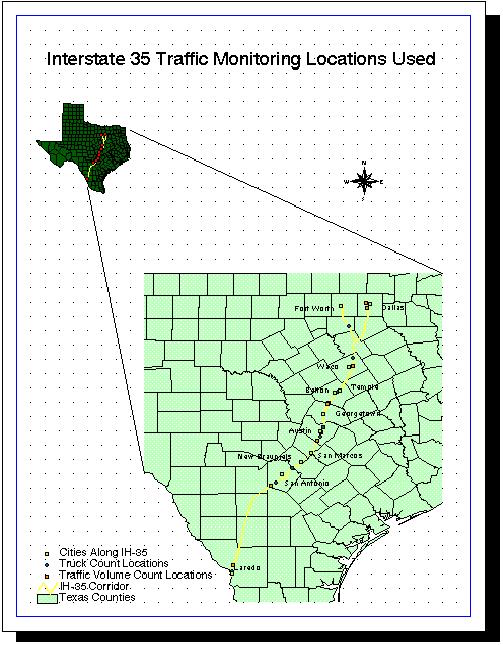
The study region was selected to be the corridor of IH 35 that extends from Dallas/Ft. Worth, Texas (35 East and 35 West) to the Mexico/United States border at Laredo, TX. This was because one of the long term goals of this project has been to establish a database for studying the effects on air quality from increased truck volume due to the North American Free Trade Agreement.
The initial shapefiles for this region were previously downloaded and made available for the students' use in either the ESRI file folders on the main hard-drive or from Dr. Maidment's ArcView data reserve. A layout was created in ArcView for the region using three main coverages.
The next GIS step was to put the traffic monitoring locations on the regional map. This was so that the locations where the traffic data were being recorded could be observed spatially, thus allowing a more educated analysis of the region. This would also enable someone to see where more data might be needed.
Two coverages were created. One coverage consisted of the permanent traffic monitoring locations along IH-35 and the other consisted of the sites where actual visual truck (over two axles) classifications were done. Both coverages were created similarly to the process presented in exercise four of the Spring 1997 GIS class. The most challenging step here was to get the location of the monitoring stations from the mileage distances along IH 35 given in the obtained data to the latitude and longitude coordinates used by the geographic projections of the other coverages. This problem was solved by using the MEASURING tool icon in ArcView with its distance set to miles. The length along IH 35 could then be measured as the lat./long. coordinates were being given on the view screen.
Here is a layout showing the addition of the monitoring locations.
The Mobile programs are considered by many to be the standard in traffic emission estimates. However, the implications of the output values from this program are not always easily seen. One of the ever increasing applications of GIS could be taking this output from the model and not only displaying the data spatially, but to aid in any calculations done with this data.
The first step in interfacing Mobile 5a to the GIS was to determine and create the sections of IH 35 that Mobile 5a was to be run for. One of the major inputs into the Mobile program is the average speed that the vehicles are traveling at. When this is calculated for the IH 35 corridor, it can be seen that there are not only varying speeds along the highway, but that in the urban areas the speeds are time dependent (e.g. the rush hours have a great effect on the urban sections of IH 35 while the rural stretches are unaffected).
One of the most convenient ways to visually display different values for different sections of the highway is to somehow label each section of concern differently in the legend. Unfortunately the sections of I35 in the original shapefile were not precise enough. The coverage for the IH 35 shapefile was originally queried from a coverage of all the major roads in the United States, and the sections of the line coverage ran from highway intersection to highway intersection. Therefore, new segmentation of the line coverage was needed
The process of segmenting a line coverage is completed in ArcInfo under the ArcEdit program. First the shapefile shown in ArcView had to be converted to a coverage using the SHAPEARC command in ArcInfo. Next, the coverage was imported into ArcEdit. Here the file was loaded by using the EDIT command. The coverage was displayed by setting the viewing window size with the MAPEXTENT command, and putting it on the screen with the DISPLAY 9999 command. The features to draw are set with the DRAWENVIRONMENT ARC command, and the actual coverage appears with the DRAW command. Presets could be set with the SNAPARC ON command, but because no intersecting lines were being worked on so it was unnecessary. Here is an example of the ArcEdit display of the interstate after the additional nodes were created.
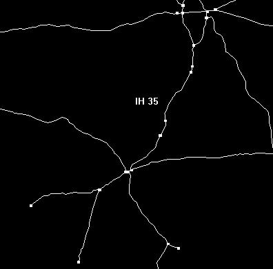
The divisions were made using the cross-hairs and coordinates that appeared when the SPLIT command was initiated. (Once again the coordinates were determined by using the measuring tool on the original layout of IH 35.) A node was automatically inserted where the divisions were made, and the attribute table was immediately updated. Finally the new coverage was converted back to a shapefile using the ARCSHAPE command in ArcInfo, and the newly segmented line coverage could be displayed in ArcView. The whole procedure for segmenting arc coverages is explained in more detail in Understanding GIS, the Arc/Info Method, by Environmental Systems Research Institute.
The IH 35 highway was divided into the twelve sections shown here.
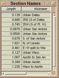
This is actually a section of the attribute table for the IH 35 corridor with the length of each segment shown.
Now that there was an acceptable segmentation of the interstate, the Mobile program had to be run for each of the sections. As mentioned before the main difference in the inputs for each section was the average speed. (The county fleet distribution was not available at the time of presenting this report.) A sample of the input and output is shown.
The next step was to take the outputs and multiply then to get the total load in grams per mile per day for each of the sections. This was accomplished by manually inputting the output data into an ArcView table and then joining this table to the already existing attribute table for the segmented IH 35 shapefile (named I35 Corridor). Here the calculation was easily performed. The final load contribution data was then easily obtainable, and it could be used to visually distinguish the different segment's pollution loading for each contaminant on an ArcView view or layout.
Here is the final table where the Mobile outputs were imported to and the final calculations were easily done in ArcView:
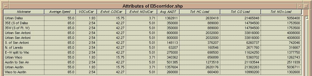
From here the following layouts were created distinguishing the road segments in the legend by their respective total daily loads in (g/mile/day). Here is the analysis layout for the NOx loading along the I35 corridor;
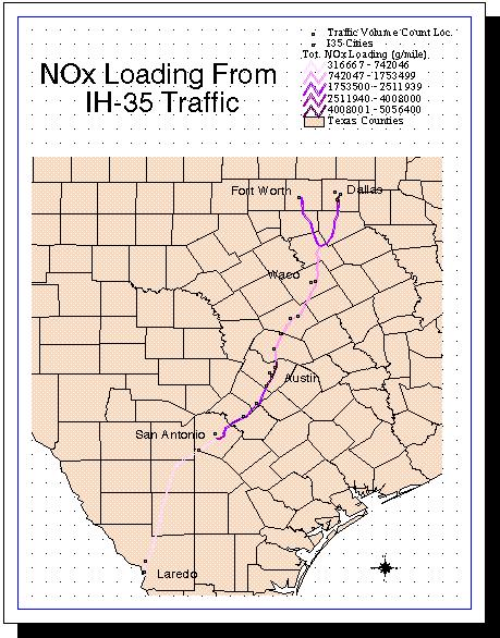
The road segments are color ramped so that the stretches of road with the lighter coloring have the smaller loadings and the darker coloring represents the heavier loadings. As can be seen by the map, the two stretches of road with the heaviest loading are the urban stretch of Austin and the urban stretch of Dallas. This corresponds to the two largest annual average daily traffic totals that were obtained from the permanent traffic monitors. The following plot shows the traffic densities and the trends of the total traffic from 1992 to 1995.
The display map for the VOC loading also has the colors ramped so that the darker the color the larger the loading is from that section of highway. One thing to note on both maps is that there is a non-intuitive amount of loading indicated on the maps for the stretch of IH 35 from Austin to San Antonio. The reason for this is because the only traffic volume data point on this section is very close to Austin. This point is probably not giving the best representation of the average flow along this section. However, this loading is left 'uncorrected' because the traffic flow here is too small for the urban section and with the acquisition of more data, the point will probably be averaged or omitted for a more realistic value.
There is still a lot of work to be done with this project. Basically it can go on for as long as I want to take it, but I do hope that I get the opportunity to see this work even further. The ultimate goal for this project would be to develop it so that the most precise emissions estimate data are taken in there GIS form and inputted into a Urban Airshed Model (UAM). This model would take into account several source inputs, but because on-road traffic is such a big part of the pollution contribution, it would be best if this input could be as precise as possible. GIS will be the major link for this input, because the analysis must be done spatially. However this is the extremely long range goal.
THE NEXT STEP....
** (This file was also used to do the final calculations before it was Joined using the JOIN command in ArcView to the I35corridor.dbf)
Hopefully this section will help you out if you ever want to run the Mobile 5a model.
Inputs:
The next line of information in the input file is the eight class breakdown (or VMT mix) of the vehicles on the road. These are Light Duty Gas Vehicles (LDGV), Light Duty Gas Trucks (LDGT, class one and two), Heavy Duty Gas Vehicles (HDGV), Light Duty Diesel Vehicles (LDDV), Light Duty Diesel Trucks (LDDT), Heavy Duty Diesel Vehicles (HDDV), and motorcycles (MC) respectively.
The next series of numbers is a breakdown by age of vehicles of each class for the past 15 years (usually). Finally the last set of numbers is giving the maximum and minimum temperatures, speeds, date, humidities, year, and other settings that may be needed depending on the input commands chosen.
Outputs:
(Again any further questions can be answered by looking at the online and down-loadable users manual at the EPA's Vehicle and Engine Emission Modeling Software page.
Understanding GIS, the Arc/Info Method, by Environmental Systems Research
Institute, Redlands, CA

FUTURE WORK

APPENDICIES
GIS Data Dictionary

Mobile 5a Data Dictionary
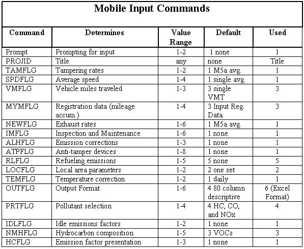
When you look at a Mobile 5a input file for the program, you first see the above commands following their number settings. Mobile 5a is was written in FORTRAN so it is very sensitive to where the input values are found. You need to be very meticulous whenever making the input file (it might be easier to start with one of the sample input files that can be downloaded from the same page as the program.)
The output file is given so that the Composite emission factor in grams/mile/vehicle are first given for each vehicle. A weighted average is then done so that the single value can be taken for each chemical for each run. This is done by adding up all the products of the classes' emissions by their percentage of the total VMT mix.
References
