Rainfall runoff in the Guadalupe River Basin
CE 397 GIS in Water Resources
by Esteban Azagra Fall 1998
Table of Contents
Introduction
MethodologyBasin Model
Precipitation Model
Control SpecificationsApplication to the Guadalupe River basin
Sources of data
Working with HEC-PrePro
Running HMS
Analyzing Parameters
Comparing resultsConclusions
Future Work
Data dictionary
Acknowledgments
References
Hydrologic Modeling System (HMS) is a computer program developed by the Hydrologic Engineering Center (HEC) of the United States Army Corps of Engineers. The program is designed to simulate the surface runoff response of a river basin to precipitation, computing the streamflow hydrographs at desired locations in the river basin. In addition to unit hydrograph and hydrologic routing options, capabilities include a linear distributed-runoff transformation that can be applied with gridded rainfall data such as ‘radar’ data, a simple moisture depletion option that can be used for simulations over extended periods, and a versatile parameter optimization option. The program works around a representation of the basin as an interconnected system of hydrologic and hydraulic components that must be introduced by the user.
HEC-PrePro is a system of Avenue scripts and controls developed by the Center for Research in Water Resources (CRWR) that allows the use of hydrologic, topographic and topologic information from digital spatial data to prepare an input file that can be read by HMS. The input file, called basin file, contains the hydrologic and hydraulic components of the basin. The use of HEC-PrePro makes the calculation of the parameters required by HMS easier and faster, improving the efficiency of the modeling system.
The objective of this project is to run HEC-PrePro/HMS for a sample area and to make a comparison between the runoff generated by the model and the field data. The final goal is the calibration of the modeling system. The sample area chosen for the study is the Guadalupe River basin.
Figure 1 resumes the methodology followed in the analysis. The first step is the inclusion of the topographic, hydrologic and topologic data into the ArcView GIS System. This information is processed by HEC-PrePro and exported into the basin file together with a series of parameters required by HMS for the calculation of the runoff. Those are the parameters that must be changed for the calibration of the system.
HMS generates the Basin Model with the information included in the basin file, which contains parameter and connectivity data for hydrologic elements. The additional information that must be introduced into HMS includes the Precipitation Model, with the meteorological data and the information required to process it, and the Control Specifications, with time-related information for a simulation.
Once the three sets of data are completed, it is possible to run HMS and
generate the runoff. The values of runoff calculated by the model can be compared with
field data and new parameters can be chosen and introduced back into modeling system. This
process should be repeated until a good calibration is achieved.
Figure 1: Methodology
One of the first tasks is the determination of the parameters that will be modified in the calibration. These parameters will be included into the basin model. The hydrologic parameters and information required by HMS can be divided in two groups. The first one corresponds to the watersheds and the second to the streams.
Watersheds. The watershed parameters determined by HEC-PrePro are area, length and slope of the longest flow-path, average curve number, and lag-time. The abstraction and routing methods chosen for this study are the ones proposed by the SCS, which require the calculation of the curve number grid from the land use data and soils data. As stated above, HEC-PrePro calculates that grid. The use of the L/V routing method requires the inclusion of a new parameter (the longest flow-path velocity) which would complicate the calibration. The analysis time-step must be supplied as input.
Streams. The stream parameters calculated by HEC-PrePro are the length, the routing method, the Muskingum K, and the number of sub-reaches into which the streams are divided in case Muskingum is used for routing, or the flow time in case pure-lag is used for routing. The use of Muskingum or pure-lag for routing depends on the length of each stream and is determined automatically by HEC-PrePro. The stream parameters flow velocity and Muskingum X must be supplied by the user.
The analysis performed on the different parameters is explained later on the document.
The precipitation model is the set of information required to define historical or hypothetical precipitation to be used in conjunction with a basin model. HMS allows several options for specifying hypothetical storms (frequency-based and the Corps of Engineers' Standard Project Storm) and historical precipitation (cell-based precipitation, previously determined spatially-averaged precipitation, specify gages and associated weights, or inverse distance-squared weighting in cases of missing data).
The first idea when this study was started was to use the gridded precipitation model that allows the use of non uniform precipitation. Typically gridded precipitation is interpreted from ‘radar’ rainfall measurements but may also be generated from gage data.
Control specifications include the starting end ending dates for a simulation, and the time interval for computations.
Application to the Guadalupe River basin
As already mentioned, the sample area chosen for the analysis is the Guadalupe River basin (see picture).
Figure 2: Sample area
The study requires GIS data and field data. Most of the data files required (mainly those corresponding to GIS data) were already available from previous works made at UT University. However, it is important to indicate the initial sources of that information.
GIS Data:
The Digital Elevation Model (DEM) necessary for delineating watersheds can be downloaded from the United States Geological Survey (USGS). DEMs are grids representing elevation of the terrain, and are available at several scales and levels of detail. The DEM used in the study is a 500 m grid cell.
The stream network used for the basin was the River Reach File 1 Coverage (RF1) from the United States Environment Protection Agency (EPA). Watershed boundaries are determined from the Hydrologic Unit Maps (HUC) developed by the USGS.
Curve numbers can be calculated from the soils characteristics included in the STATSGO database developed by the U.S. Department of Agriculture (USDA), and the Land Use/Land Cover (LULC) data developed by the United States Environment Protection Agency (EPA).
Field Data:
Precipitation data should be obtained from NEXRAD measurements in the National Climatic Data Center (NCDC).
Finally, information regarding stream flow measurements is available from the USGS gage stations.
A typical sequence of work with HEC-PrePro starts with the delineation of watersheds and the stream network definition. The first step consists in "burning in" the RF1 stream network into the DEM. Next is the filling of the sinks of DEM to avoid problems calculating the flow direction. Figure three shows the grids corresponding to those steps.
Figure 3: DEM, "Burning in" and Fill Streams grids.
Once those pits have been filled, it is possible to calculate the flow
direction and the flow accumulation grids, represented in Figure 4. These steps had
already been done in the Exercise 3 of the
course "GIS in Water Resources" and it was not necessary to repeat them.
Figure 4: Flow direction and Flow Accumulation grids.
The construction of the basin stream network starts with the definition of the threshold
or minimum drainage area. The HEC-PrePro function CRWR-PrePro/Stream Definition
(Threshold) prompts a dialog box to introduce a value for the threshold. The first
value attempted was 5,000 in order to reduce the number of sub-basins and streams and,
therefore, the number of parameters to manage. The result was 89 sub-basins and same
number of streams. However, the methodology followed makes unnecessary the change of each
parameter individually. Thus, the final threshold selected was 1,000.

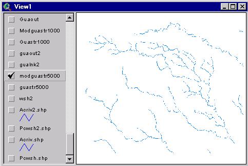
Figure 5: Basic Stream Network (thresholds 1000 and 5000).
Following, is the creation of a point coverage of flow gauging stations. The idea is to create a table with the name of the stations and the coordinates in longitude and latitude (expressed in decimal degrees). This table can be imported into ArcView, creating a shape file with points representing the gage stations. It is necessary to use the CRWR-Vector/Project function to project the gages locations from Geographic into USGS National Albers Projection. and it is important to ensure that the gages are located over streams. This can be checked using the zoom feature of ArcView. If necessary, a new point close to the gage but over the stream can be added with the O button.
Next steps are the segmentation of streams into stream links with the CRWR-PrePro/Segmentation (Links) function, and the determination of the watershed outlets with the CRWR-PrePro/Outlets from links and CRWR-PrePro/--Add Outlets functions. This function also allows definition of outlets in those points of the streams where the gages are located, and not only in the most downstream cells of each stream segment.
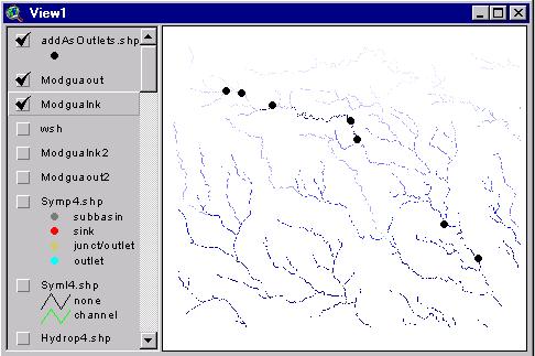
Figure 6: Gauges, outlets and links.
Starting with the above grids and with the CRWR-PrePro/Sub-Watershed Delineation function, it is possible to delineate the sub-watersheds. The next step is the vectorization of streams and watersheds, converting their raster representation into a vector representation. The function used for this task is CRWR-PrePro/Vectorize Streams and Watersheds. The result is a polyline shape file with streams and another one with the watersheds. Figure 7 shows how the delineated sub-watershed basin looks like as well as the shape files resulting from the vectorization.
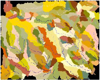
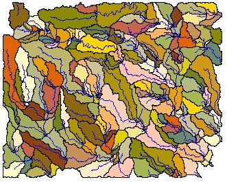
Figure 7: Watersheds and streams (before and after vectorization).
The SCS method used for the calculation of the lag-time requires the inclusion of the average SCS curve number of the sub-basin. This value is determined as an average of the curve number values within each sub-basin polygon. A curve number grid has been calculated from the Anderson Land Use Code and the STATSGO soils data, using the HEC-PrePro functions CRWR-PrePro/Soil (Group Percentages) and CRWR-PrePro/Curve Number Grid.
Up to this point, all the pre-process of the hydrologic system is finished. The next step is the calculation of the hydrologic elements parameters for each element, that will be attached to their corresponding attribute tables and exported to HMS into the basin file. This is achieved running the HEC-PrePro function CRWR-PrePro/Calculate Attributes. HEC-PrePro asks for the abstraction and lag-time methods to be used. As we already mentioned, the selected methods in both cases are the proposed by the SCS. A warning window reminds the user the requirement of a curve number grid for the methods selected. Another warning indicates the requirement of an input file with the stream velocity and the Muskingum X. This file will change while different parameters are used in the calibration but, in any case, its structure will be similar to the one showed on Figure 8.
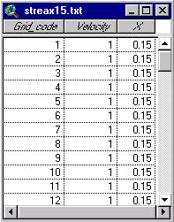
Figure 8: Example of parameter table.
The last part before running HMS is the isolation of the Guadalupe River
basin (using the C button), the calculation of the schematic, and the generation of
the basin file for HMS. The last two steps are accomplished with the CRWR-PrePro/HMS
Schematic function. The result is stored in four shape files and one text files that
can be used by HMS.
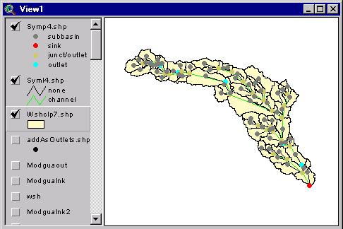
Figure 9: Guadalupe Basin Schematic.
HMS generates the Basin Model with the information included in three data sets: the Basin File, the Precipitation Model and the Control Specifications.
The basin file is automatically created by HEC-PrePro and can be loaded into HMS without any change. The result appears in Figure 10.
Two different Precipitation models have been used in the project. The first one is a hypothetical precipitation value introduced with the Frequency-Based Hypothetical Storm method. This value has been used to analyze the influence of the different parameters in the calibration. The first idea was to use a Grid-Based Precipitation from 'radar' data, but it was not possible to find the information required. Therefore, precipitation data corresponding to the USGS stations selected for the study was downloaded from the Internet and introduced into HMS as a User-Specified Hyetograph. Details are explained later.
Finally, Figure 11 shows an example of the Control Specifications used in
the part of the study corresponding to the analysis of parameters.
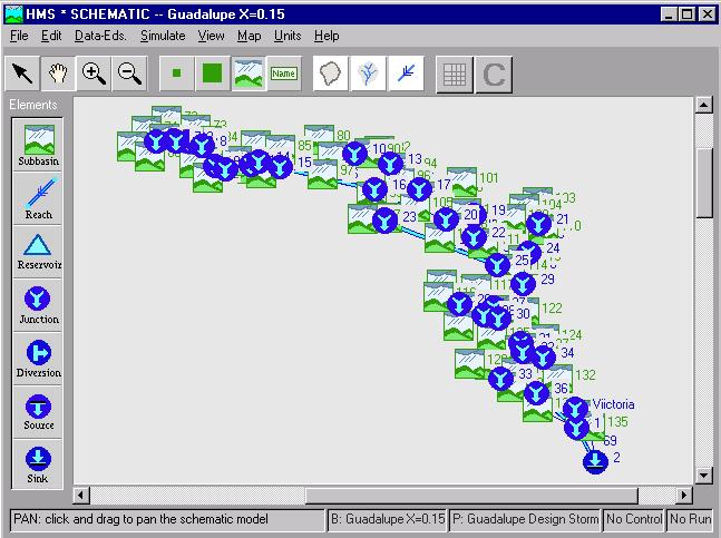
Figure 10: HMS Schematic the for Guadalupe River Basin.
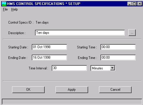
Figure 11: HMS Control Specifications.
There has been performed an analysis of the parameters involved in the modeling process to determine the relative importance of each one in the modelation. It was already mentioned that, with the abstraction and routing methods chosen for the study, there are three parameters that must be supplied as input by the user: the analysis time-step, the stream flow velocity and the Muskingum X.
The analysis of the parameters has been done by using the Precipitation Model showed in Figure 12. The values correspond to a hypothetical storm.
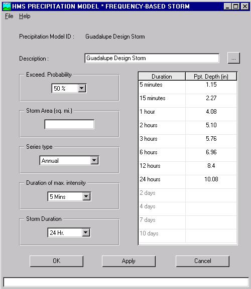
Figure 12: HMS Precipitation Model for a hypothetical storm.
The value corresponding to the analysis time-step has been fixed to 30 minutes. This ensures that Muskingum is used for routing in more than 95% of the streams, a value considered correct for this kind of studies.
The next variable analyzed is the Muskingum X. Three modeling sessions have been accomplished keeping the stream velocity fixed at 1 m/s, and values of X equal to 0.15, 0.20 and 0.25 respectively. Results show that, for a variation of 20% in the value of X (considering that 0 < X < 0.5), the peak outflows measured at one location -in this case Victoria Station- vary around 3.7 %. It is easy to see that great accuracy in determining X may not be necessary because the results will be relatively insensitive to the value of this parameter.
On the other hand, keeping the Muskingum X fixed at 0.20, and trying values of the stream velocity equal to 0.8, 1.0 and 1.2 m/s, the peak outflows measured at the same location present variations up to 28 % (considering a range of velocities between 0 and 2 m/s).
Figure 13 shows the results of both calculations.
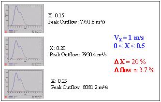
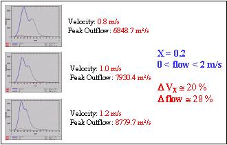
Figure 13: Analysis of X and Vx variables.
It is clear that the variable of interest for the study is the stream velocity, since its weight in the final runoff is much bigger than the corresponding to X. The calibration should be accomplished by changing the velocity and keeping the Muskingum X fixed at 0.2, which is a correct value for natural streams.
The total number of streams generated by HEC-PrePro within the Guadalupe
Basin using a threshold of 1,000 is 89. In order to make changes in streams velocities
easier, the problem has been approached using the Manning's formula ![]() . The parameter
. The parameter![]() includes both the Manning's
number n and the hydraulics radius R, and S represents the slope of the stream. This
approach is not completely correct because the hydraulic radius varies from one stream to
another, and in the study
includes both the Manning's
number n and the hydraulics radius R, and S represents the slope of the stream. This
approach is not completely correct because the hydraulic radius varies from one stream to
another, and in the study ![]() has been considered equal for all streams. However, this simplification
can be assumed in order to ease the task.
has been considered equal for all streams. However, this simplification
can be assumed in order to ease the task.
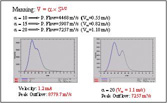
Figure 14: Vx variation for different values of alpha.
Another simplification assumed in this study is the use of the longest flow path's slope
within each sub-basin assuming that it is the one corresponding to the stream of the
sub-basin (note that no sub-basins have been merged and, therefore, each sub-basin has
just one stream within it).
The precipitation data available for the study to create the User-Specified Hyetograph model has been obtained from records corresponding to the seven USGS gages selected for this study. The problem is that data found corresponds to daily values of precipitation and streamflows.
All gage data associated with the project has been entered manually via the Gage Data option on HMS. The data introduced includes the precipitation used to develop precipitation hyetographs for sub-basins and also streamflow data used to define discharge for a source hydrologic element, for optimization of basin model parameters, and for comparison with simulated streamflow.
Once precipitation data has been entered, it is necessary to relate each gage with the corresponding sub-basins (that whose assigned precipitation is the value measured in the gage). The ArcInfo function Thiessen helps determine which sub-basin corresponds to which gage. This function creates a Thiessen Polygon coverage from the locations of the precipitation stations. A more detailed explanation of Thiessen polygons applications can be found in the Term Project "Concentration of Chemicals of Concern in the soil Matrix for the Marcus Hook Refinery", written by Aiza Jos�. Figure 15 shows the result after using the function.

Figure 15: Thiessen polygons.
The input of the sub-basins and associated gages has also been done manually through the User-Specified
Hyetograph screen shown in Figure 16. The process has been quite long because names of
the hydrologic elements are assigned randomly by HEC-PrePro and it has been necessary to
find out which name was assigned to each of the 64 sub-basins.
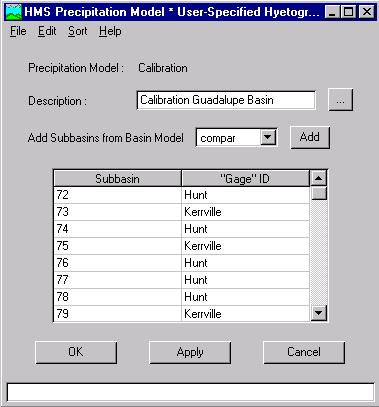
Figure 16: User-Specified Hyetograph input screen.
The model has been run with the referred data for a fifteen days period, between
06/20/1997 and 07/04/1997, and three values of alpha (10, 15 and 20). There was a big
storm the week selected for the study and it has been possible to find some information
relative to the time when it happened. This information has been used to make a time
distribution of the precipitation registered. Figure 17 shows the hydrograph corresponding
to Victoria gage generated by HMS for a value of alpha equal to 10.
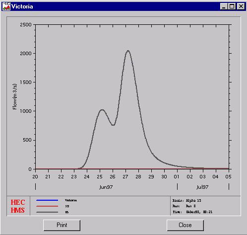
Figure 17: Hydrograph at Victoria.
Although it is not possible to make the accurate comparison required for the calibration
of the model, some aspects of interest can be analyzed from the results obtained.
The peak outflow occurs on June the 27th with a value between 2079.4 cms and 1964.4 cms, depending on alpha. There is a time delay of the event for decreasing values of alpha, something logic because we are decreasing the velocity of the water. The model also predicts an smaller flow peak on June the 25th. The total discharge calculated by HMS is 472,572,000 cu m.
Field data show that the biggest value for the mean flow occurred the 23rd of June, four days before the peak outflow predicted, with 566 cms registered. Assuming the biggest mean flow occurs the same day than the maximum peak flow, we can see that the model is delaying the event.
The total discharge measured at Victoria can be determined from the mean values of the flow times the number of days. The result is 418,435,200 cu m. This means the model is predicting a discharge 11.5 % bigger than the real one.
Small values of stream velocities (alpha) could delay the peak flow predicted by the model but will not have the incidence shown by the results. The differences caould be explained by a wrong time distribution of the precipitation. With daily values it is not easy to determine at what time of the day precipitation occurred.
Nevertheless, the differences on the total discharge are not very significant if we consider that the number of gages was not very high (they were initially selected to control de flow at different points of the streams, not as a source of information for precipitation data). This means that the use of Thiessen polygons to obtain a distribution of precipitation is very useful and accurate.
Although the final goal of the project has not been fulfilled because the field data available was not appropriate, the study shows that modeling runoff with the help of GIS can be an effective tool to characterize watersheds. Provided the proper information it will be possible to obtain satisfactory results.
The methodology proposed to calibrate the model by changing just one parameter is fast and could be a convenient approach to the problem. However its efficiency was not proved in this study.
Calibration using gauging data must be attempted selecting more gauging stations in order to increase accuracy. The identification of the sub-basins corresponding to each gage should be done automatically.
Most important is the use of NEXRAD precipitation data. This would increase the resolution and precision of the studies. This data must be converted to a DSS file before being imported to HMS, and it would be very useful to make the process automatically. There is already a lot of work done in those directions by the CRWR.
Finally, a calibration can be done using the watershed lag-time calculation method. This method requires the inclusion of the longest flow-path velocity. Using two parameters instead of just alpha could perform the analysis. The longest flow-path of each sub-basin and the corresponding slope are already calculated by HEC-PrePro, but it may be necessary to modify the script used for these calculations in order to calculate the slope of the streams in each sub-basin. With this, one of the simplification used in this study would be avoided.
| Acriv | Polyline shape file of streams generated after the vectorization of streams. |
| addAsOutlets | Shape file with the corrected flow gauging station theme. |
| Addlines | Shape file of streams consistent with the flow direction grid (guafdr). |
| alpha##.txt | Tables of stream hydrologic parameters. |
| Burned1 | Grid of DEM with streams GuaRF1 burned on it. |
| Calibration.precip | HMS file with the precipitation model used for the calibration. |
| Cn | Curve number grid of the Guadalupe basin. |
| Comp.dbf | dBase attribute table of Statsgo for Texas. |
| Dem | Grid of digital elevation model (DEM) for the Guadalupe basin region. |
| Design_Storm.precip | HMS file with the precipitation model used for the analysis of parameters. |
| Gageprj | Shape file with a point theme of the USGS gauging stations selected. |
| Gages.dbf | Table of flow gauging stations along the Guadalupe river. |
| glu | Shape file of the Guadalupe land Use from USGS Land Use/Land Cover files. |
| Gs | Clipped version of Statsgo for the Guadalupe basin. |
| Guabasin##.basin | Text files generated by HEC-PrePro which are the basin files required by HMS. |
| Guadalupe##.run | HMS files with the Simulate/Run configurations. |
| Guadalupe_Basin.dss | DSS file generated automatically by HMS for the simulation. |
| Guadalupe_Basin.gage | HMS file with the stream flow and precipitation data of the gages. |
| Guafac | Grid of flow accumulation of a digital elevation grid (Guafill). |
| Guafdr | Grid of flow directions of a digital elevation grid (Guafill). |
| Guafill | Grid of filled digital elevations (Burned1). |
| Guahuc | Shape file of the Hydrologic Cataloging Units in the Guadalupe basin. |
| Gualnk | Grid of stream segments in a stream grid (Modguastr1000). |
| Guaout | Grid of watershed outlets defined as the most downstream cell of each segment of a stream segment grid (Gualnk). |
| Guarf1 | River reach file for the Guadalupe Basin. |
| Guastr1000/Guastr5000 | Grid of streams for a threshold of 1000/5000 cells in a flow accumulation grid (Guafac). |
| hecdiv.dbf | Table for attribute transfer from ArcView shape files to HMS basin files. |
| hecjunct.dbf | Table for attribute transfer from ArcView shape files to HMS basin files. |
| hecreach.dbf | Table for attribute transfer from ArcView shape files to HMS basin files. |
| hecres.dbf | Table for attribute transfer from ArcView shape files to HMS basin files. |
| hecsink.dbf | Table for attribute transfer from ArcView shape files to HMS basin files. |
| hecsourc.dbf | Table for attribute transfer from ArcView shape files to HMS basin files. |
| hecsub.dbf | Table for attribute transfer from ArcView shape files to HMS basin files. |
| Hydrol#.shp | Shape files generated by HEC-PrePro with hydrologic information necessary for HMS. |
| Hydrop#.shp | Shape files generated by HEC-PrePro with hydrologic information necessary for HMS. |
| Layer.dbf | dBase attribute table of Statsgo for Texas. |
| Mapunit.dbf | dBase attribute table of Statsgo for Texas. |
| Modgualnk | Grid of stream segments calculated after the inclusion of the gauging stations as outlets. |
| Modguaout | Modified grid of watershed outlets with the gauging stations included. |
| Modguastr1000 | Grid of streams that combines into one a grid of streams (Guastr1000) with a shape file of streams (Addlines). |
| Pcwsh | Polygon shape file of watersheds generated after the vectorization of watersheds. |
| Prepro03.apr | Project file with the Scripts, Menus and Buttons for running CRWR-PrePro. |
| Rivclp# | Shape files with the stream lines themes corresponding to the streams of the Guadalupe basin only. |
| SEVEN_DAYS.control | HMS file with the control specifications used for the calibration. |
| slopes.xls | Microsoft Excel Worksheet used for management of alpha##.txt files. |
| Statsgotx | Shape file of Statsgo for Guadalupe basin. |
| StreamP.txt | Tables of stream hydrologic parameters. |
| Syml#.shp | Shape files generated by HEC-PrePro with hydrologic information necessary for HMS. |
| Symp#.shp | Shape files generated by HEC-PrePro with hydrologic information necessary for HMS. |
| TEN_DAYS.control | HMS file with the control specifications used for the analysis of parameters. |
| Thiesn | Shape file generated using Thiessen Polygons, with the precipitation area corresponding to each gage. |
| vector10.avx | CRWR-Vector extension file. |
| wsh | Grid of subwatersheds delineated for each outlet in Modguaout. |
| wshclp# | Shape files with the polygon themes corresponding to the watershed polygons of the Guadalupe basin only. |
| WshPar.txt | Tables of watershed hydrologic parameters. |
The contribution of Francisco "Paco" Olivera, Brian Adams and Kwabena Asante, who helped me diminish my doubts is greatly appreciated.
Chow, V.T., Maidment, David R. and Mays, L.W. / Applied Hydrology. / New York, 1998.
Hydrologic Engineering Center. / HEC-HMS Hydrologic Modeling System, Program User's Manual. / U.S. Army Corps of Engineers, Davis, California, 1998.
Maidment, David R. / Handbook of hydrology. / New York, 1993.
Olivera, F., Reed, S. and Maidment, D. / HEC-PrePro v. 2.0: An ArcView PreProcessor for HEC's Hydrologic Modeling System. / Center for Research in Water Resources, Austin, Texas, 1998.
Prepared by Esteban Azagra
4 December 1998