A few commercial software companies have capitalized on this opportunity. BOSS International currently distributes RiverCAD software that allows users to display HEC-RAS output in AutoCAD. However, it is our understanding that Geographic information systems (GIS) offer a superior environment for this type of work. Although CAD is a good environment for visualization, GIS provides tools for more complex queries, storage, mapping, analysis, and visualization of the spatial data. Recognizing the advantages of GIS, Dodson & Associates, Inc. has developed GIS Stream Pro, with which the user can develop HEC-RAS cross-sections based on a terrain model. After running HEC-RAS, GIS Stream Pro can delineate the floodplain in ArcView GIS. GIS Stream Pro requires the user to input parameters in HEC-RAS, such as Manning coefficients, bridge and culvert descriptions, and channel contraction/expansion coefficients. For a large HEC-RAS model, this could require a large amount of time for model development. But more importantly, most terrain models do not represent streams very well, due to interference from trees and water in the photogrammetry process. So will cross-sections developed from a terrain model contain sufficient resolution for hydraulic modeling in HEC-RAS?
Many practicing engineers already have established HEC-RAS models for floodplain analysis. The tools described in this tutorial offer a method by which to quickly post-process HEC-RAS output, to allow floodplain visualization and analysis in ArcView GIS. Also, the method can be used develop a terrain model with a high density of points in the channel and a lower density elsewhere. Thus, this single terrain is usable for both hydrologic and hydraulic modeling.
The data required for this exercise consist of an HEC-RAS output data file, ArcView shapefiles, and digital imagery, which can be downloaded as two zip files. Floodmap1.zip is a 0.5 MB file that contains the HEC-RAS and ArcView files. Floodmap2.zip is a 7.2 MB file containing digital orthophotography. The data will be used in this tutorial to construct a digital floodplain map of Waller Creek, located in Austin, Texas. Specifically, the zip files contain the following data:
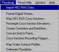
Summarized descriptions of these menu items are provided as follows:
A. Data Import
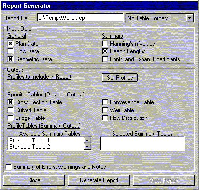
When you are finished setting up the window, click the "Generate Report" button. HEC-RAS will subsequently create an output file and save it in a location you designate. The resulting output file can be viewed in any text editor. Note the location where you saved the file, and exit HEC-RAS.
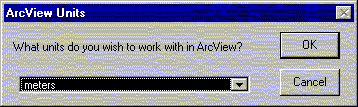
Next we will import the HEC-RAS data into our ArcView project. Go to the view window and select the Floodmap/Import HEC-RAS Data menu option. Before continuing, it is necessary to choose the units you'd like to work with. For this tutorial, the HEC-RAS model has units of feet. However, the GIS data (shapefiles, orthophotography, and DEM) are in units of meters. When queried by ArcView for the units, select meters:
Depending on the size of the output file and the speed of your computer, the import process could take
anywhere between a few seconds to a couple of minutes. The progress is shown at the bottom of the view
window. When the processing is complete, select a file name and location when prompted. Basically, this
step transforms the output data from textfile format into dBASE format, which can be read by ArcView as
a table. To view the data in ArcView, return to the main project window and click on the
 icon. The table selection window should now show "Table1." Open it and your
window should appear something like this:
icon. The table selection window should now show "Table1." Open it and your
window should appear something like this:
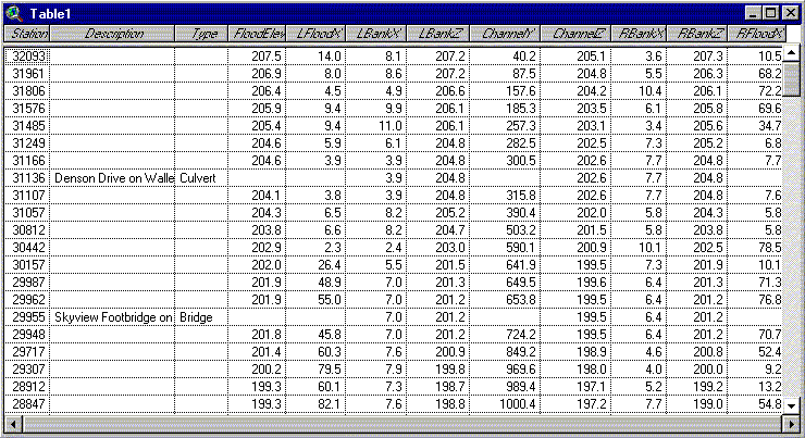
For each cross-section in the HEC-RAS output file, the following data has been retrieved and stored (the text in parenthesis refers to the table column name):
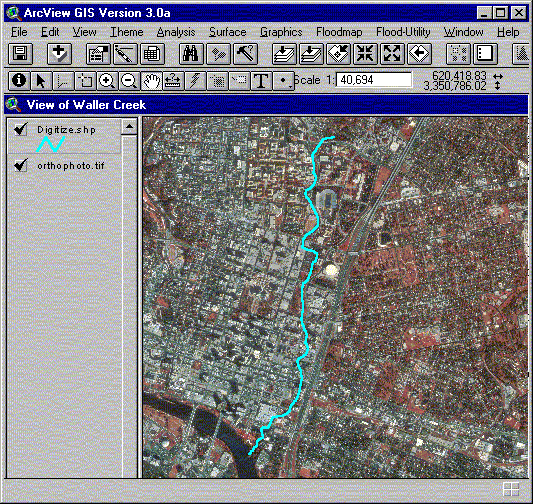
 , the add theme button. After making sure that the data source type in the add
theme window is set to "Feature Data Source", choose digitize.shp. To provide some perspective, also
use the button to open the digital orthophoto, orthophoto.tif. To do so, make
sure the data source type in the add theme window is set to "Image Data Source." The view window should now
look like this:
, the add theme button. After making sure that the data source type in the add
theme window is set to "Feature Data Source", choose digitize.shp. To provide some perspective, also
use the button to open the digital orthophoto, orthophoto.tif. To do so, make
sure the data source type in the add theme window is set to "Image Data Source." The view window should now
look like this:
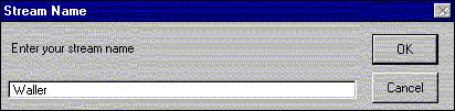
Regardless of the source of the stream centerline, the attribute table of the shapefile will need to be modified to allow its use in subsequent steps of the floodplain mapping. To do so, make the digitized line theme active, and select Floodmap/Format Digital Stream. When prompted for the stream name, enter "Waller":
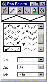
We no longer need the theme digitize.shp, so you may delete it from the view window. At this point, it is important to know the direction of the stream line theme. Although common sense says that it should point upstream to downstream, HEC-RAS defines streams in the opposite direction. To be consistent with the HEC-RAS data, the digital stream should point from downstream to upstream. To check the direction of the line, double click on the theme in the legend bar in order to bring up the legend editor. Click on the pen palette and choose an arrow representation.
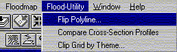
In actuality, Waller Creek flows from north to south. In this case the digital stream is oriented correctly, from downstream to upstream. If this wasn't the case, the direction could be reversed by making the theme active, and selecting Flood-Utility/Flip Polyline.
To help define the upstream, downstream, and intermediate points, we'll use a theme of Austin roads in the
point delineation process. Click on the button and add the theme roads.shp. In the
legend bar, activate the roads theme and click on its checkbox to view it. Then select Theme/Auto-label.
The following window should appear:
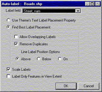
As the label field, select "Street_nam" and click OK. The roads theme will now be labeled with the individual
street names. Next activate waller.shp in the legend bar, and click on the  tool. We're
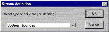
now ready to start defining points on the digital stream. The points we will define are as follows:
tool. We're
now ready to start defining points on the digital stream. The points we will define are as follows:
| Location | Type |
|---|---|
| 26th Street | Upstream Boundary |
| MLK Blvd. | Intermediate Point |
| 15th Street | Intermediate Point |
| 11th Street | Intermediate Point |
| 7th Street | Intermediate Point |
| 1st Street | Intermediate Point |
| End of Waller Creek | Downstream Boundary |
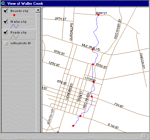
You can display the roads theme and/or the orthophoto to help locate the definition points. But for now, we'll just use the roads theme. So turn of the orthophoto theme in the legend bar. To begin, find the intersection of 26th Street and Waller Creek, and click the mouse at that spot. When queried for the type of boundary, select "Upstream boundary."
The click of the mouse causes the script attached to the tool to determine
the nearest point along the stream centerline and snap the point onto the digital stream. Next
find the intersection of MLK Blvd. and Waller Creek and define it as an intermediate point. Proceed
to define the rest of the points, moving from upstream to downstream. The view window should now
look like:
The stream definition points will form the backbone of the cross-section georeferencing process. Using the data table resulting from the data import step, the HEC-RAS data corresponding to the definition point locations will be associated with these map coordinates. For example, the table record for Waller Creek at 11th street will be connected with the definition point located at Waller Creek at 11th street. This concept is illustrated in the following graphic:
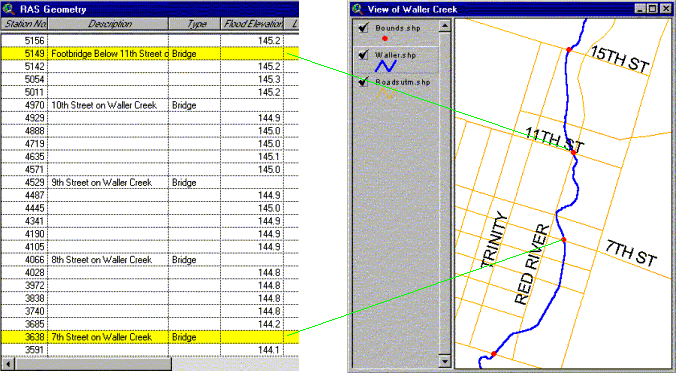
To select the relevant HEC-RAS data, return to Table1. Using the "Station" and "Description" columns as a guide, highlight the record for 26th Street at Waller Creek (Station 13167). Scroll down to select the remaining six records, holding down the shift key to select more than one record.
| Definition Point | "Station" | "Description" |
|---|---|---|
| 26th Street | 13167 | 26th Street on Waller Creek |
| MLK Blvd. | 8920 | Footbridge Below MLK on Waller Creek |
| 15th Street | 7148 | 15th Street Bridge on Waller Creek |
| 11th Street | 5149 | Footbridge Below 11th Street on Waller Creek |
| 7th Street | 3638 | 7th Street on Waller Creek |
| 1st Street | 1198 | Cesar Chavez on Waller |
| End of Waller Creek | 0 | --- |
When finished, click on the  tool to promote the highlighted records to the
top. Check them to make sure you've selected the correct seven records. Now return to the view window
and select Floodmap/Map HEC-RAS Cross-Sections. (Note: It is important that this step is
performed in the same sitting as the data import step. Otherwise, you'll receive the error message
"A(n) nil object does not recognize the request get." This is because much of the cross-section data
is stored in global variables, which are not saved with the project when exiting ArcView.) When
queried, choose "Bounds.shp" as the stream definition point theme, Waller.shp as the stream centerline
theme, and Table1 as the HEC-RAS geometry table. One of the query windows will appear as follows:
tool to promote the highlighted records to the
top. Check them to make sure you've selected the correct seven records. Now return to the view window
and select Floodmap/Map HEC-RAS Cross-Sections. (Note: It is important that this step is
performed in the same sitting as the data import step. Otherwise, you'll receive the error message
"A(n) nil object does not recognize the request get." This is because much of the cross-section data
is stored in global variables, which are not saved with the project when exiting ArcView.) When
queried, choose "Bounds.shp" as the stream definition point theme, Waller.shp as the stream centerline
theme, and Table1 as the HEC-RAS geometry table. One of the query windows will appear as follows:
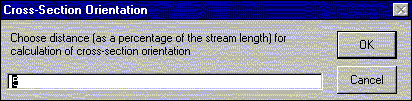
This input window is for a parameter that will determine the orientation of the cross-section relative to the stream centerline. Using a value of 0 will cause each cross-section to be mapped perpendicular to the stream, at the precise cross-section location. Using a zero value could cause some cross-sections to intersect near bends in the stream. As the orientation parameter increases, perpendicularity is determined based on a longer segment of the stream. For this tutorial, use the default value of 5.
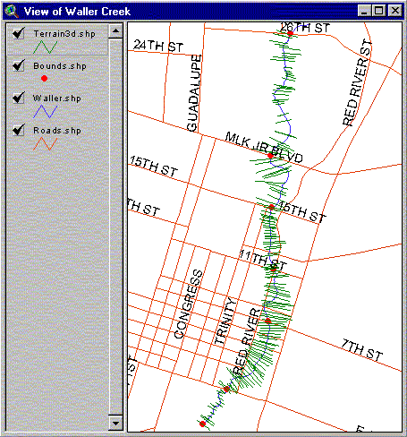
The resulting line theme of the HEC-RAS cross-sections should appear like the graphic shown above. You'll notice that each of the cross-sections is represented as a straight line. In reality, some of the cross-sections may have been set up as doglegs. However, this information is not stored in HEC-RAS, and as such, the straight line assumption was made. At this point, it would be a good idea to save the ArcView project.
Creating a TIN terrain model from two different data sources presents its challenges: the DEM and HEC-RAS data have different collection times, methods, and resolutions. So at the point where the HEC-RAS data ends and the DEM data begins, called the transition zone, some elevation differences are expected. A method to smooth the transition zone is applied. For each cross-section, between the stream banks and the ends, the elevations are resampled using elevation values from the DEM. To initiate this process, add the 30-meter DEM to the view. We'll need to do some work on the DEM before continuing. For some reason, many DEMs are constructed with latitude and longtitude measured in meters and elevation measured in feet. This is the case with our data set. To remedy this, first select Analysis/Properties. Set both the Analysis Extent and Analysis Cell Size to "Same as Auseast." Click OK and select Analysis/Map Calculator and set up the window as shown below:
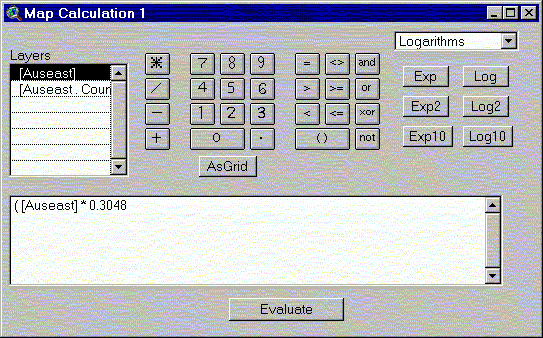
After clicking OK, a new grid will be created, this time with the elevations in meters. Highlight the new grid in the legend bar, and save the new grid under the name "auseast1" by selecting Theme/Save Data Set. Although you've given the new DEM a name, the legend bar will still show "Map Calculation 1." You can change the legend bar name by selecting Theme/Properties.
We're now ready to begin the terrain modeling. Select Floodmap/Re-Sample Cross-Section Elevations. When queried, choose "Terrain3d.shp" and "auseast1" as the inputs. This process could take a few minutes--the elevation of every cross-section point outside of the main channel is being recalculated. To help visualize the result of the cross-section resampling, a tool with which to create three profiles of any given cross-section has been developed, based on the original cross-section, the DEM, and the resampled cross-section. Select Flood-Utility/Compare Cross- Section Profiles. Select the appropriate themes and the cross-section (river station) you'd like to profile. I've used river station 2510. The coordinate data is written to an ASCII text file that can be plotted using Microsoft Excel. Save the text file and open it in Excel. The Excel text import wizard should engage. The text file is comma delimited, so click next and in the second window check the comma box, followed by the finish button. With the data now in a spreadsheet, they can be graphed on an x-y scatter plot:
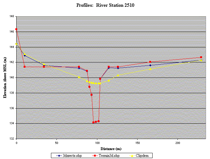
There are two things to be noted about this plot:
Now we will work on the DEM data. To create a TIN with ArcView 3D Analyst, the input data must be either raster or vector, but not both. So we'll perform a raster to vector conversion on the DEM. Because the DEM is much larger than our study area of Waller Creek, it will be clipped to a smaller size. Open the theme "polyclip.shp" from your working directory. The DEM will be clipped to the extent of this polygon theme. Now select the Flood-Utility/Clip DEM menu item, and use "30mDEM" as the grid and "polyclip.shp" as the clipping theme. Now we are ready for the raster to vector conversion. Select Floodmap/Convert Grid to Points to convert the clipped DEM to a point shapefile.
As input for our terrain TIN, the cross-sections will represent areas within the floodplain and the DEM points will provide elevations for the landscape outside the floodplain. A polygon bounding the cross-sections will be used to delineate the transition zone between the two data sources. To form the polygon, select Floodmap/Cross-Sections Bounding Polygon and choose "3dxsects.shp" as the line theme. At this point, the view window should look somewhat like the following graphic:
The final step before creating the TIN, is to eliminate any DEM points falling within the
cross-sections bounding polygon. We can identify these points by intersecting the DEM point
theme with the bounding polygon. Make the bounding polygon theme ("Boundary.shp") active
and highlight it using the  tool. Next make the DEM point theme
("Gridpt.shp") active and select Theme/Select by Theme. Using the drop-down lists,
make the window look like the following graphic and click on the "New Set" button.
tool. Next make the DEM point theme
("Gridpt.shp") active and select Theme/Select by Theme. Using the drop-down lists,
make the window look like the following graphic and click on the "New Set" button.
Click on the  button to go view the attribute table of the DEM point theme.
In the table window click on the and all of the selected point records
to the top. We'll now edit these points out of the shapefile. Select Table/Start Editing
and then Edit/Delete Records. Now select Table/Stop Editing and save the edits.
If you now return to the view window, you'll notice that the DEM points only occur outside
of the floodplain. We're now ready to create the terrain TIN. In the legend bar, make active
the themes "Stream3D.shp", "3dxsects.shp", and "gridpt.shp". Then select Surface/Create
TIN from Features and the following window should appear:
button to go view the attribute table of the DEM point theme.
In the table window click on the and all of the selected point records
to the top. We'll now edit these points out of the shapefile. Select Table/Start Editing
and then Edit/Delete Records. Now select Table/Stop Editing and save the edits.
If you now return to the view window, you'll notice that the DEM points only occur outside
of the floodplain. We're now ready to create the terrain TIN. In the legend bar, make active
the themes "Stream3D.shp", "3dxsects.shp", and "gridpt.shp". Then select Surface/Create
TIN from Features and the following window should appear:
The theme "Stream3d.shp" is a three-dimensional line shapefile of the stream centerline and banklines. These data will be enforced in the TIN as breaklines. Fill in the window as shown in the graphic. Next, click on the cross-section line theme "3dxsects.shp" on the left side of the window. In the "Input as:" drop down list, select "Mass Points." Finally, click on the DEM point theme, "Gridpt.shp." Select "Mass Points" from the "Input as:" window and "Grid_code" as the "Height Source." Now click the OK button to create the TIN. When ArcView has finished processing the data, the TIN theme will appear in the legend bar. Click the check box to display it. The default color scheme is not ideal for observing the TIN. Double click on the TIN's legend bar to open the TIN legend editor. First click off the check box next to "Lines" and then click the edit button in the "Faces" part of the window. This will open the regular legend editor. Click on the Load button and choose "land.avl." Click OK in the Load Legend" window and then apply in the legend editor. (The image captured from the screen is much grainier than the actual image in ArcView.)
Make the TIN theme active and use the  to query the elevations at
different locations. Notice that there is a smooth transition where the hydraulic data
(cross-sections) meets the DEM data. To view the TIN in 3D, select View/3D Scene
and add the view as Themes when queried. To maneuver in the 3D scene, click and hold the
left mouse button while moving the mouse. The time required to render the image will depend
on your computer's processor speed, RAM, and video card. The right mouse button can be used
to zoom in and out. By clicking and holding both mouse buttons, the pan tool is enabled.
to query the elevations at
different locations. Notice that there is a smooth transition where the hydraulic data
(cross-sections) meets the DEM data. To view the TIN in 3D, select View/3D Scene
and add the view as Themes when queried. To maneuver in the 3D scene, click and hold the
left mouse button while moving the mouse. The time required to render the image will depend
on your computer's processor speed, RAM, and video card. The right mouse button can be used
to zoom in and out. By clicking and holding both mouse buttons, the pan tool is enabled.
You now have a TIN that depicts the general landscape, but also has additional detail in the stream channel and floodplain. The density of points within the channel is sufficient for hydraulic modeling. A terrain model such as this could be used as an input for software such as GIS Stream Pro.
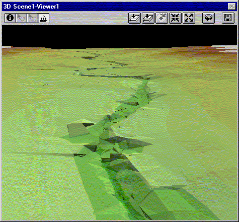
The water surface line theme can be used to create a TIN model of the floodwater surface. If the HEC-RAS model was set up correctly, the water surface extent will not exceed the cross-section extent. As such, the cross-section bounding polygon will serve as the outer boundary of our water surface TIN. Activate the water surface theme ("Water3d.shp") and the bounding polygon theme ("Boundary.shp") in the legend bar and select Surface/Create TIN from Features. In the TIN creation window, input the water surface theme into the TIN as hard breaklines, and the bounding polygon theme as a hard clip polygon and then click OK. The default color scheme really doesn't look much like floodwater, so if you like, you can load the legend named "water1.avl." When viewed in a 3D scene in conjunction with the terrain TIN, flooded areas can be seen:
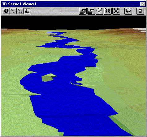
The three-dimensional floodplain view is quite useful for floodplain visualization. But the view shown in the graphic doesn't appear much like the actual landscape. To remedy this, 3D Analyst allows the addition of themes of roads, buildings, railroads, etc., that can be draped over the landscape to more closely approximate reality.
For detailed analysis, the floodplain can be viewed from a planimetric perspective, using a basemap such as a digital orthophotograph. But in order to be accurate, inundated areas should not be delineated using the terrain TIN. Why? The HEC-RAS water surface profiles used to create the water surface TIN were determined using the original cross-sections and not the resampled cross-sections. Hence, a new TIN of the surface terrain needs to be constructed. Activate the themes "Terrain3d.shp", "Stream3d.shp", and "Gridpt.shp" in the legend bar, and select Surface/Create TIN from Features. Specify the parameters just as before in the Terrain Modeling section and click OK. At this point, you can delete resampled cross-section line theme ("3dxsects.shp") and its associated terrain TIN from the view.
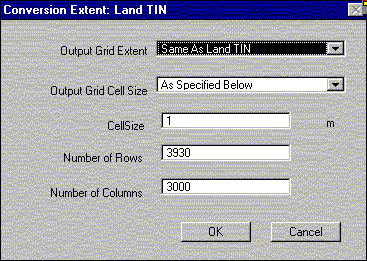
Now we have a TIN model for both the land surface and the floodwater. However, the floodplain delineation is more readily performed using the raster data model instead of TINs. In the raster domain, grid cells of water surface elevation and grid cells of land surface elevation can be easily compared using map algebra. As such, we need to convert both TINs to grids. Make the land TIN active and select Theme/Convert to Grid. Choose "landgrid" when prompted for a grid name. In the conversion extent window, set the Output Grid Extent to be the same as the land TIN, set the Output Grid Cell Size to "As Specified Below," and input the cell size as 1 meter:
After clicking OK, ArcView will convert the TIN to a 1-meter resolution grid. Do the same for the water surface TIN. But this time, name the grid watergrid and set the Output Grid Extent to be the same as the water surface TIN. Now both surfaces are represented as grids. Before comparing the two grids, it's necessary to define the analysis extent. Select Analysis/Properties. Set the Analysis Extent to Same as Watergrid, set the Analysis Cell Size "As Specified Below" and input it as 1 meter. Then select Floodmap/Delineate Floodplain. The script will compare the two grids and create an output grid consisting only of areas where the floodwater elevation exceeds the land surface elevation. For the floodplain grid, the color scheme "water2.avl" can be loaded from the legend editor. Add the orthophoto to the view as a basemap:
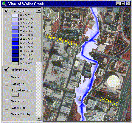
You now have a floodplain map, in which the extent of flooding can easily be compared to
structures of interest shown on the orthophoto, such as businesses, schools, and homes. In
addition, the tool can be used to query the depth of flooding at
any point in the floodplain.
Go to Eric Tate's Home Page