PHOTOGRAMMETRY APPLICATIONS IN
DIGITAL TERRAIN MODELING AND FLOODPLAIN MAPPING
For my master's research in civil engineering, I am developing procedures to connect hydraulic modeling output to geographic information systems (GIS). When the approach is finalized, a hydraulic engineer should be able to take a set of water surface profiles computed through hydraulic modeling, and map the associated floodplain in GIS. During the course of my research, I have discovered that a significant component of GIS floodplain mapping involves building an accurate digital terrain representation of the study area, Waller Creek. Important inputs to the digital terrain representation are digital orthophotographs and digital terrain models. The techniques used to develop these data are based on principles of photogrammetry.
Photogrammetry is defined as the science or art of obtaining reliable measurements by means of photography (Thompson, 1966). Although the term can apply to measurements from ground photographs, modern photogrammetric techniques are most often applied to aerial and satellite images. One of the most common uses of photogrammetry is the analysis of aerial photography to extract ground elevations for the production of topographic maps. However, the field also includes the production of digital orthophotographs and digital terrain models. This paper focuses on the procedures used to develop these digital data and their applications to my research.
The first half of the paper is devoted to the photogrammetric techniques used to develop digital orthophotographs and digital terrain models. The topics covered include image acquisition, stereoscopic parallax, digital terrain model development, and digital orthophotographs.
The first step in the production of digital orthophotograph and terrain models is capturing aerial photographs of the land surface. To acquire the images, a plane travels over a study area in a straight flight line, and photographs are taken such that every ground point appears in at least two successive photographs. The resulting photos are called a stereo pair, and the area of common coverage is called overlap. If the study area of interest requires more than one flight line for complete coverage, additional flight lines are flown parallel to the original line. Overlap between adjacent flight lines is called sidelap, and is used to prevent gaps in coverage. Standard overlap is 60% forward and 15% side (Figure 1).
Figure 1. Image Coverage using Overlapping Photographs
Figure 2. Example of a raster digital image
Typically, aerial photographs designed for digital orthophotograph production are taken with a camera with a 6-inch focal length lens, at an altitude of 15,000 feet; this generates photographs with a scale of 1:30,000. The film diapositives (transparencies) are later scanned with a precision image scanner to create a digital raster image file. Although the resulting raster images appear to be continuous, in reality they consist of a grid of discrete uniformly sized square cells.Each cell, or pixel, is assigned a gray scale value that corresponds to the average intensity of the ground area covered by the pixel (Lillesand, 1994). Figure 2 shows how a raster digital image might appear if shown as gray scale values. As the resolution of the scanned image increases, magnification is required to discern the individual pixels with the naked eye.
Methods of visually judging depth may be classified as either stereoscopic or monoscopic (Wolf, 1974). Monoscopic vision refers to viewing surrounding objects with only one eye. Depth is perceived primarily based on the relative sizes of objects and hidden objects; distant objects appear smaller and behind closer objects. However, depth perception is poor with monoscopic vision, and distance estimation can be difficult. In stereoscopic vision, objects are viewed with both eyes, producing a composite three-dimensional image. Stereoscopic vision allows for a far greater degree of depth perception than monoscopic vision. The concept of stereoscopic vision can also apply to viewing an aerial photography stereopair. By viewing the left photograph with the left eye and the right photograph with the right eye, a three-dimensional view of the terrain can be obtained (Lillesand, 1994). An instrument called a stereoscope is designed to aid in this type of visualization. Many people will find stereoscopic viewing of aerial photography without a stereoscope to be quite a challenge.
Parallax is the apparent displacement in the position of a stationary object, with respect to a frame of reference, caused by a shift in the position of observation (Wolf, 1974). If an object is observed monoscopically with the left eye and then the right, there is an apparent shift in position. As the distance between the observer and object decreases, the apparent position shift increases. An instrument called a stereometer is used to measure differences in parallax between objects in a stereopair. Parallax equations can then employed to convert measured parallax into object height.
Based on the definitions given above for stereoscopic vision and parallax, the term stereoscopic parallax refers to perception of depth based on viewing objects from separate points of observation. Stereoscopic parallax is a very important concept in photogrammetry because it allows for the measurement of height of objects appearing a stereopair.
A model of the surface terrain can be developed using an analog instrument called a stereoplotter. The primary use of stereoplotters is for the production of topographic maps. The typical stereoplotter is composed of components for light projection, stereopair viewing, and tracing terrain features:
To plot the position of a given point, the tracing table is be raised or lowered until the dot appears to rest on the ground. Ground control points (x,y,z) established based on ground surveys or aerial triangulation are viewed in the stereoplotter in conjunction with the stereo pair. In this setting, the image coordinates of (x,y,z) points in the stereo pair are determined and randomly selected and recorded.
The stereoplotter described above is an analog instrument. Most photogrammetrists today instead use digital image processing software to extract terrain elevations from aerial photography. However, the point extraction process is quite similar, with the notable exception that the stereopair is viewed in the computer as a scanned raster image. Using the processing software, the photogrammetrist selects and digitizes a high density of points. The selected image coordinates, in conjunction with the ground control points, comprise the data points used to construct a digital terrain model.
A triangular irregular network (TIN) model is typically used to digitally represent the terrain surface. A TIN is a triangulated mesh constructed on the (x,y) locations of a set of data points. To form the TIN, a perimeter around the data points is first established, called the convex hull. To connect the interior points, triangles are created with all internal angles as nearly equiangular as possible. This procedure is called Delaunay triangulation. By including the dimension of height (z) for each triangle vertex, the triangles can be raised and tilted to form a plane. The collection of all such triangular planes forms a representation of the land surface terrain in a considerable degree of detail.
Figure 3. Triangular Irregular Network Surface Representation
Additional elevation data such as spot elevations at summits and depressions and break lines can also be included in the TIN model. Break lines represent significant terrain features like a lake or cliff that cause a change in slope; TIN triangles do not cross break lines.
The elevation points extracted from the stereomodel can also be used to create a raster (grid) model of terrain elevations. A land surface representation in the raster domain is called a digital elevation model (DEM). However, the TIN model is typically preferred for three-dimensional surface representation because a TIN requires a much smaller number of points than does a grid in order to represent the surface terrain with equal accuracy.
Digital orthophotos are scale correct aerial photographs. Conventional aerial photographs have limited use for making measurements because they are not true to scale. When you look at the center of an aerial photograph, the view is the same as if looking straight down from the aircraft. However, the view of the ground toward the edges of the photograph is from an angle. This is called a central perspective projection; scale is true at the very center of the aerial photograph, but not elsewhere. In order to create a scale correct photograph that can be accurately measured, an orthographic projection is necessary, in which the view is straight down over every point in the photograph.
The procedure used to create digital orthophotographs, called ortho- rectification, requires aerial photography and an associated TIN digital terrain model as inputs. The TIN surface is used to orthogonally rectify the scanned raster image file. By combining the TIN and raster image, each image pixel is attributed with a known location and intensity value. In the rectification process, the intensity value for each pixel is re-sampled using a space resection equation, thus removing image displacements caused by central perspective projection, camera tilt, and terrain relief. The individual photographs are then clipped and seamlessly joined together over the entire study area. The result is a digital image that combines the image characteristics of a photograph with the geometric qualities of a map--a true to scale photographic map. The resulting ground/pixel resolutions can be finer than 1 foot. However, the accuracy of the final digital orthophotograph depends in large part on the point density of the TIN terrain model.
Digital orthophotos have many uses in the GIS environment. Some orthophotograph benefits include the following:
May be used as a GIS base map for a variety of uses, including urban and regional planning, revision of digital line graphs and topographic maps, creation of soil maps, and drainage studies
More cost effective and display more surface features than conventional maps
Easily available over the internet from the U.S. Geological Survey (USGS) or the Texas Natural Resources Information System (TNRIS)
Digital orthophotographs available from USGS and TNRIS are tied to North American Datum (NAD) 1983 in the Universal Transverse Mercator projection. Each digital image covers the same area as a USGS 7.5-minute quadrangle topographic map, but is divided into four parts. Hence, the final product is called a digital orthophotograph quarter quadrangle (DOQQ).
Up to this point in the paper, the discussion has focused on the development of digital terrain models and digital orthophotographs through photogrammetry. In the next section, the application of these digital data to my research in GIS floodplain mapping is detailed.
Figure 4. Waller Creek in Austin, Texas
As part of the research, digital orthophotographs were used as a base map for two-dimensional floodplain mapping, and a TIN digital terrain model was developed to aid in three-dimensional floodplain visualization.
Before creating a floodplain map in GIS, the output data for the stream of interest must first be extracted from the hydraulic model and imported into ArcView. Upon completion of this intial step it is necessary to associate the modeled stream with same stream in digital form. There are two primary ways to obtain a digital representation of a stream:
Both digital data sources were evaluated for the research. However, digital orthophotos were found to provide a more accurate spatial representation of Waller Creek than did RF3. This determination did not come as much of a surprise; the RF3 hydrography was developed by digitizing water bodies from topographic maps that could be decades old, whereas the flights to develop the TNRIS digital orthophotographs were performed in 1995. As such, 1-meter resolution orthophotography for the Austin East USGS 7.5-minute quadrangle was obtained from TNRIS. In ArcView, the image for the southwest DOQQ was used as a base map on which to digitize Waller Creek (Figure 5).
As part of the mapping process, some key points along Waller Creek were also digitized. These points identify the upstream and downstream boundaries used for the hydraulic modeling and intermediate stream definition points corresponding to important cross-sections such as bridges or culverts. Often, these points were more easily pinpointed by comparison to the location of an existing structure (e.g., road, bridge, etc). As such, a base map theme of roads was used in addition to the digital orthophoto to assist in the point selection process.
Figure 5. Stream mapping using a digital orthophotograph base map
After mapping the floodplain, zoom tools in ArcView allow the hydraulic engineer to easily compare the location of the floodplain versus the locations of structures of interest, such as buildings and roads (Figure 6). The digital orthophotograph base map allows the landscape surrounding the floodplain to be viewed as it really appears, producing a far superior backdrop than could be expected from a scanned paper map.
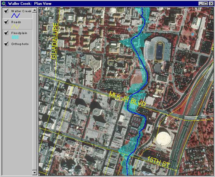
Figure 6. Floodplain mapping with a digital orthophotograph base map.
The floodplain map shown in Figure 6 is detailed enough to be used for measurement of floodplain extent. But data describing floodplain depth would also be useful. This type of analysis requires a three-dimensional rendering of the floodplain. For three-dimensional floodplain visualization, an accurate TIN terrain model is crucial. The best TIN will include as much input elevation data as possible. To provide for regional terrain elevations, a 30-meter DEM was downloaded from the TNRIS website. Elevation data from the hydraulic model was used to describe the channel and floodplain of Waller Creek. Construction of an integrated terrain TIN from these data requires the combination of the high-resolution hydraulic model elevation data with comparatively low-resolution DEM data. This task is complicated by the fact that the two data types are of different structures: the DEM data is of the raster domain, while the stream data consist of vector objects.
Vector objects in a GIS include three types of elements: points, lines, and polygons. A point is defined by a single set of Cartesian coordinates (x,y). A line is defined by a string of points in which the beginning and end points are called nodes, and intermediate points are called vertices (Smith, 1995). A straight line consists of two nodes and no vertices whereas a curved line consists of two nodes and a varying number of vertices. Three or more lines that intersect to form an enclosed area define a polygon. Vector feature representation is typically used for linear feature modeling (roads, lakes, etc.), cartographic base maps, and time-varying process modeling.
The vector objects used to describe Waller Creek consisted of numerous cross-section lines, and three lines representing the stream centerline and the left and right banks. The DEM was used to for elevations outside the floodplain. By combining the vector and raster data to form a TIN, the intended result is a continuous three-dimensional landscape surface that contains additional detail in stream channels. The approach is illustrated in Figure 7.
The procedure includes the following steps:
Using these steps, a three-dimensional terrain TIN can be constructed such that the floodplain elevation data supersedes the DEM data within the area for which it is defined and the DEM elevations prevail elsewhere, with a smooth zone of transition. Once the terrain model is complete, it is fairly simple to add the flood water to the terrain surface to enable floodplain visualization.
At present, my research stands at step 6: smoothing the interface between the raster and vector data sources. A TIN was created, but the zone of transition is quite ragged (Figure 8). Based on the known differences between the DEM and floodplain elevation data, this result was expected. The floodplain elevation data is an amalgamation of field surveys and topographic map estimations over a period of 10-15 years in the 1970's and 1980's. The DEM was formed from the digital terrain model used to develop the TNRIS digital orthophotographs in 1995. Given that the data have different collection times, methods, and resolution, it was not surprising that they would be incompatible. However, elevation differences of up to 25 feet between data sources were observed at some points, suggesting error in one or both of the data sets.
Figure 8. Preliminary three-dimensional terrain model
As an attempt to identify the flawed data, an additional data source was employed. In November, the Capital Area Planning Council CAPCO) released spot elevation data for the City of Austin and several surrounding counties. The resulting elevation data was the result of a large photogrammetry project performed from 1996 to 1998. I obtained the CAPCO data for Waller Creek, and created a TIN from these elevations in ArcView in an effort to use it as an independent data source to check the accuracy of the integrated TIN. The CAPCO TIN had a very high resolution, with data points every foot in some places. As such, it was assumed to be more accurate than my TIN. In comparing the two, it was discovered that the DEM data over-estimated elevations outside the channel, whereas the vector data underestimated them, each by approximately 5 to 10 feet. Fortunately, the vector data elevations agreed with CAPCO results within the stream channel. My work over the next couple months will involve repairing the ragged zone of transition.
Once the TIN surface is completed, additional features can be added to allow the surface to more closely approximate reality. These features might include roads and building footprints. ArcView GIS allows these data to be draped over the TIN surface for three-dimensional visualization.
Building elevations can be measured from the digital orthophotograph based on shadow length. The calculation requires one known building height (Avery, 1992):

Where: hn = height of building n
Ln = shadow length of building n
Figure 9 shows the level of detail that can be obtained by building a detailed TIN surface model. The view shows the Colorado River south of downtown Austin. The figure was prepared using remotely sensed data compiled for the CAPCO photogrammetry project.
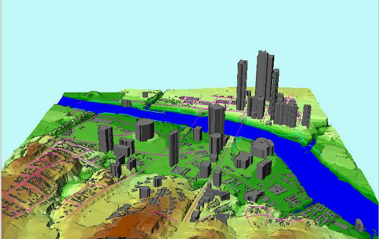
Figure 9. Surface model ultimate goal.
Overall, photogrammetry has shown itself to be a vital source of information for my research project. In fact, most of the work could not be performed without the digital data developed using photogrammetric techniques described in this paper. Digital orthophotograph data were used as a base map as background imagery, as a basemap with which digitize Waller Creek and key stream points, and to estimate building height. Digital terrain model data were used as inputs to a TIN model, and to create the CAPCO TIN used to validate my work in three-dimensional terrain modeling. As a result of this project and course, I have gained a great deal of respect for photogrammetrists and the work they perform.
